NVIDIA GPU Deep Dive : Tensor and Ray Tracing Cores

Nvidia GPU Tensor Core Architecture

This blog is Part 3 in our Nvidia GPU blog series. In Parts 1 and 2, we explored the fundamentals of NVIDIA GPU architecture: from CUDA cores to streaming multiprocessors (SMs) and warp schedulers. Today, we transition into what sets modern NVIDIA GPUs apart-the Tensor Cores and Ray Tracing (RT) Cores-two hardware innovations that fuel cutting-edge advancements in AI computation and real-time rendering.

NVIDIA Tensor and Ray Tracing Cores have revolutionized , making GPUs the backbone of deep learning workloads. Meanwhile, RT Cores enabled real-time photorealistic graphics, redefining visual realism in games and simulations. In this post, we dissect their architectures, working principles, and how they seamlessly integrate into the GPU pipeline.


🧠 Tensor Cores – Unleashing AI Performance

Architectural Evolution and Integration

Tensor Cores were introduced in the Volta (GV100) architecture, setting a new benchmark for AI acceleration. Each Streaming Multiprocessor (SM) houses multiple Tensor Cores, tightly coupled with CUDA cores and other functional units. This co-location allows Tensor Cores to offload matrix-heavy operations like convolutions and fully connected layers, while CUDA cores handle scalar/vector instructions.

Across architectures:

  • Volta: First appearance; FP16 precision support.
  • Turing: Added INT8 & INT4 precision for inference workloads.
  • Ampere: Introduced TF32 and enhanced sparsity support.
  • Hopper: Revolutionized with FP8 and the Transformer Engine.

Each SM includes hardware schedulers that coordinate the execution of Tensor Core operations alongside traditional CUDA threads, ensuring maximal occupancy and throughput.

Nvidia GPU Tensor Cores

Precision Modes: FP32, FP16, TF32, INT8, FP8, and FP4

Precision is critical in balancing performance and numerical stability.

  • FP32: Full precision; used in scientific computing.
  • TF32: Ampere’s innovation, offering FP32 dynamic range but with FP16 compute efficiency-achieves up to 10× speedup in deep learning training.
  • FP16 (Half Precision): Ideal for neural nets tolerant to low precision; critical in deep learning inference.
  • INT8 & INT4: Efficient for low-latency inference, especially on edge devices.
  • FP8 & FP4: Next-gen precision; FP8 is central to Hopper’s Transformer Engine, while FP4 is emerging for ultra-low-power inference.

Tensor Cores dynamically downscale or upscale precision based on kernel requirements, facilitated by NVIDIA’s cuDNN and TensorRT libraries.
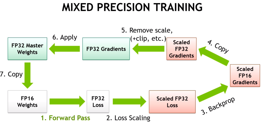
NVIDIA GPU - mixed precision training
NVIDIA GPU – mixed precision training

In-Depth: Matrix Multiply-Accumulate (MMA) Engine

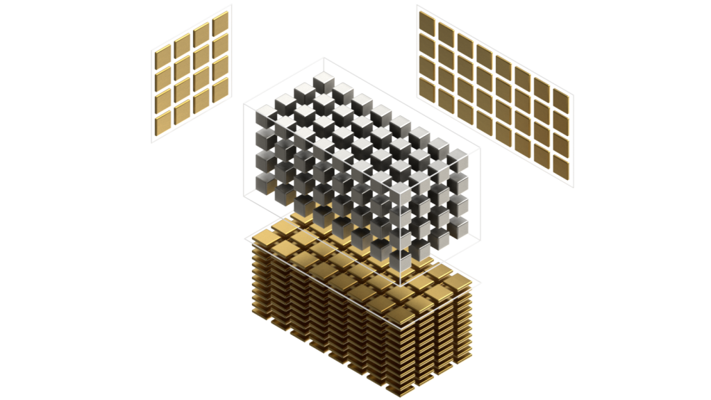
At the heart of Tensor Cores is the Matrix Multiply-Accumulate (MMA) Engine. The MMA pipeline is designed to perform:

D=A×B+C

For matrix tiles (commonly 16×16). The Tensor Core parallelizes these tiles across multiple hardware lanes, enabling:

  • 16×16×16 FP16 MMAs in a single cycle (Volta-Ampere).
  • Dynamic 8×8 tiles with FP8 in Hopper for optimized attention layers.

Tensor Cores rely on warp-level primitives, where threads in a warp collaborate on MMA operations. NVIDIA’s CUDA WMMA API provides direct access to these functionalities.


Transformer Engine & Sparsity Acceleration

Transformer models-which power LLMs like GPT-have unique computational patterns. Hopper’s Transformer Engine:

  • Detects per-layer precision requirements (FP16 vs FP8).
  • Dynamically adjusts execution precision at runtime.
  • Leverages context-aware sparsity, which identifies zero-value weights and skips redundant computation.

This enables 50%+ reductions in compute/memory without sacrificing accuracy. Ampere introduced 4:2 structured sparsity, doubling throughput for sparse models.


🎮 Ray Tracing Cores – Enabling Cinematic Real-Time Ray Tracing

The Shift from Rasterization to Path Tracing

Rasterization dominates traditional graphics pipelines by projecting 3D geometry into 2D fragments. However, it fails to simulate true light behavior like global illumination and caustics. Ray tracing simulates:

  • Primary rays (camera → scene)
  • Reflection/refraction rays (mirror/glass)
  • Shadow rays (light occlusion)

RT Cores were introduced in Turing, transforming ray tracing from a batch process to a real-time application.
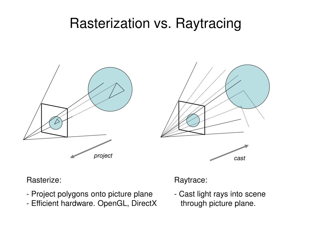
Rasterization vs Raytracing

BVH Traversal and Intersection Hardware

The core of RT Core acceleration lies in BVH (Bounding Volume Hierarchy) traversal.

  • BVH Tree: Scene geometry is hierarchically partitioned into boxes.
  • Traversal: RT Cores quickly determine if rays intersect bounding boxes-rejecting entire regions early.

Once inside a leaf node, Ray-Triangle Intersection units calculate precise hit points using barycentric coordinates and optimized hardware pipelines.

Performance: RTX 3090 achieves 10 billion BVH tests/sec, enabling complex environments at playable frame rates.


Multi-Stage Ray Shading Pipeline

The shading pipeline includes:

  • Ray Generation Shader: Initiates rays.
  • Closest Hit Shader: Determines material/shader logic on hit.
  • Any Hit Shader: Early exits for transparency effects.
  • Miss Shader: Background/environment mapping.

Each ray potentially spawns secondary rays, making recursive traversal necessary. Tensor Cores assist by AI-denoising noisy samples-enhancing visual quality without full sampling.


🤝 Tensor + RT: DLSS and Hybrid Workloads

DLSS (Deep Learning Super Sampling) epitomizes the synergy of Tensor + RT Cores. The workflow:

  1. RT Cores: Render base frame (lower resolution).
  2. Tensor Cores: Upscale + reconstruct via AI models.

DLSS 3.0 (Ada Lovelace) even predicts in-between frames using motion vectors + optical flow estimation-massively boosting FPS in ray-traced environments.

This hybrid method achieves 4K quality at 1080p costs, revolutionizing graphics performance.


🧪 Developer Toolkit: Leveraging Tensor & RT Cores

For AI:

  • CUDA WMMA API
  • cuBLAS/cuDNN
  • TensorRT

For Graphics:

  • Vulkan/DXR
  • NVIDIA OptiX
  • Nsight Visual Profiler

Profiling tools allow warp-occupancy tracking, Tensor Core utilization, and RT core tracing, helping developers fine-tune performance.


📈 Conclusion

NVIDIA’s Tensor and Ray Tracing Cores are cornerstones of modern GPU architecture, unlocking unprecedented capabilities across AI, graphics, and simulation. These specialized cores complement general CUDA compute, enabling applications that were infeasible a decade ago.

In Part 4, we’ll unravel the mysteries of GPU memory subsystems, cache hierarchies, and NVLink/NVSwitch-crucial for multi-GPU scaling.

Deep Dive into GPU Compute Hierarchy

Modern NVIDIA GPUs are feats of hierarchical design, optimized to maximize parallelism, minimize latency, and deliver staggering computational throughput. Building upon Part 1, which introduced the high-level architecture of NVIDIA GPUs, this is Part2 – a Deep dive into GPU Compute Hierarchy: Graphics Processing Clusters (GPCs), Texture Processing Clusters (TPCs), Streaming Multiprocessors (SMs), and CUDA cores. Understanding this hierarchy is essential for anyone looking to write optimized CUDA code or analyze GPU-level performance.


1. Graphics Processing Clusters (GPCs)

1.1 Overview

At the top of NVIDIA’s compute hierarchy lies the Graphics Processing Cluster. A GPC is an independently operating unit within the GPU, responsible for distributing workloads efficiently across its internal resources. Each GPC contains a set of Texture Processing Clusters (TPCs), Raster Engines, and shared control logic.

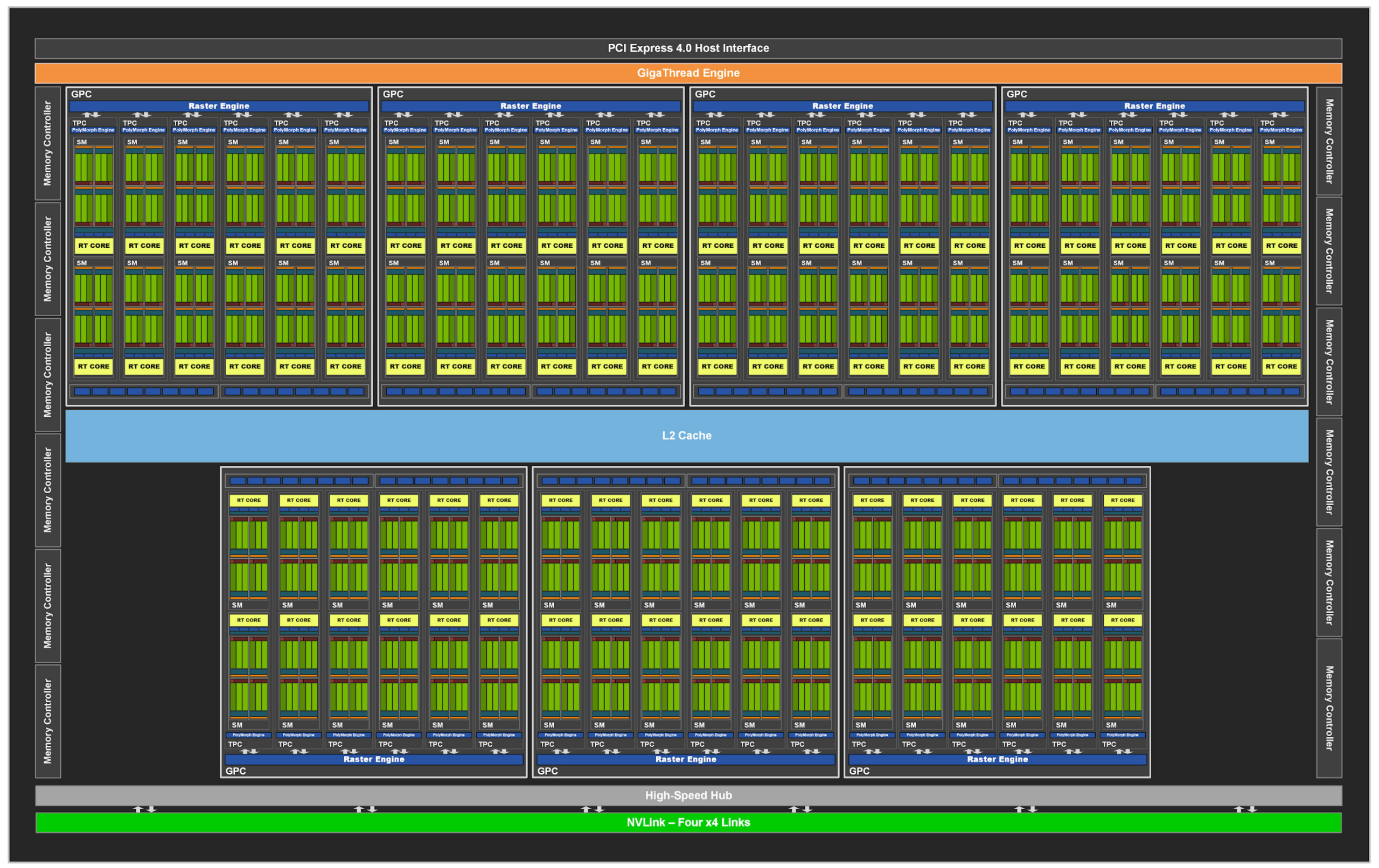
📊 GPC Block Diagram:

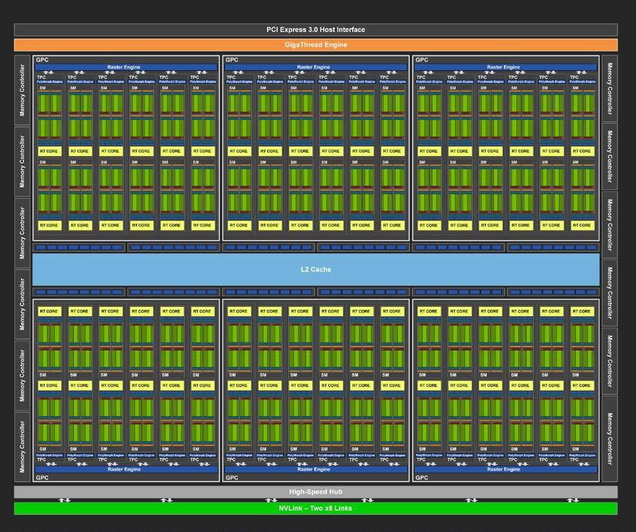
Nvidia Turing TU102 Full GPU with 72 SM Units.
Nvidia Turing TU102 Full GPU with 72 SM Units. Image : developer.nvidia.com
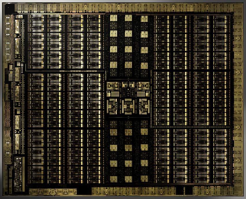
Internal Die layout of Nvida Turing TU102 GPU .
Internal Die layout of Nvida Turing TU102 GPU . Image : developer.nvidia.com

1.2 GPC Architecture

Each GPC includes:

  • One or more Raster Engines
  • Several TPCs (typically 2 to 8 depending on the GPU tier)
  • A Geometry Engine (in graphics workloads)

📘 Example GPC layout in RTX 30 series:

Nvidia RTX30 GPC block Diagram
Nvidia RTX30 GPC block Diagram. Image: Nvidia Ampere GA102 GPU Architecture document

1.3 Scalability Role

More GPCs generally equate to more parallel compute and graphics capability. High-end GPUs like the H100 feature many GPCs to support large-scale AI workloads, while mobile GPUs may only include one or two.


2. Texture Processing Clusters (TPCs)

2.1 Role of TPCs

TPCs are the next level down. A TPC groups together Streaming Multiprocessors (SMs) and a set of fixed-function texture units, providing both compute and graphics acceleration. Originally optimized for texture mapping and rasterization, TPCs in modern GPUs support general-purpose compute as well.

2.2 Components of a TPC

Each TPC typically contains:

  • Two Streaming Multiprocessors (SMs)
  • Shared L1 cache
  • Texture units (for graphics and compute shaders)
  • A PolyMorph Engine (responsible for vertex attribute setup and tessellation)

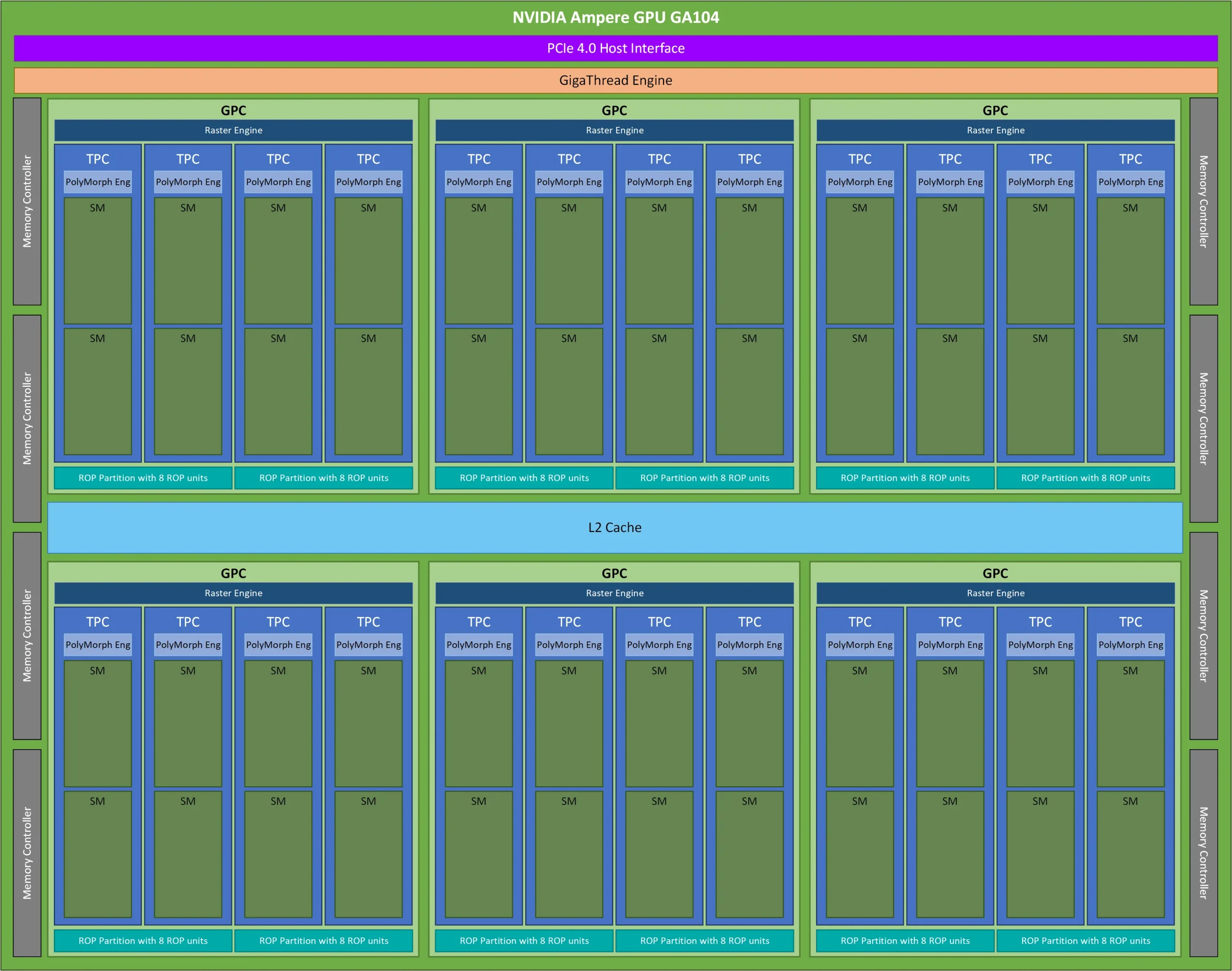
📊 TPC Diagram with SMs and Texture Units:

NVIDIA Ampere GA104 architecture showing GPC, TPC, SM.
NVIDIA Ampere GA104 architecture showing GPC, TPC, SM. Image: wolfadvancedtechnology.com

2.3 Texture Mapping

Texture units in the TPC fetch texels from memory, perform filtering (e.g., bilinear, trilinear), and handle texture addressing. These units have been extended to support texture sampling for compute workloads, such as in scientific visualization.


3. Streaming Multiprocessors (SMs)

3.1 Importance of SMs

Streaming Multiprocessors are the core programmable units of NVIDIA GPUs. They execute the majority of instructions, including floating-point arithmetic, integer operations, load/store instructions, and branch logic.

3.2 SM Internal Structure

A modern SM (e.g., in the Hopper H100 or Blackwell B100) consists of:

  • Multiple CUDA cores (up to 128 per SM)
  • Load/Store Units (LSUs)
  • Integer and Floating Point ALUs
  • Tensor Cores (for matrix operations)
  • Special Function Units (SFUs)
  • Warp schedulers and dispatch units
  • Register files
  • Shared memory and L1 cache

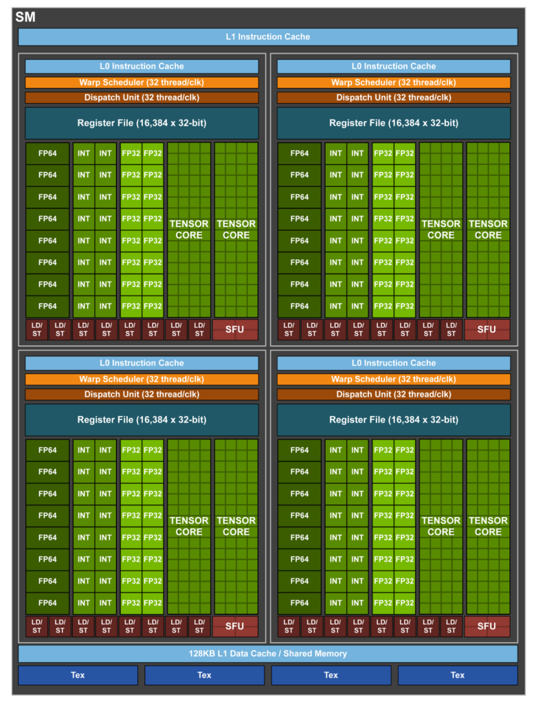
📘 SM Layout Reference (Volta/Hopper SMs):

Nvidia Volta Streaming Multiprovessor (SM) block diagram
Nvidia Volta Streaming Multiprovessor (SM) block diagram. Image: Nvidia Volta Architecture Document

3.3 Warp Scheduling

The warp scheduler picks a ready warp from a warp pool and issues an instruction every clock cycle. Techniques like GTO (Greedy Then Oldest), Round-Robin, or Two-Level scheduling are used.

Key Benefits:

  • Latency hiding: Warps can be swapped out when memory access stalls occur.
  • Concurrency: Independent warps can issue instructions simultaneously.
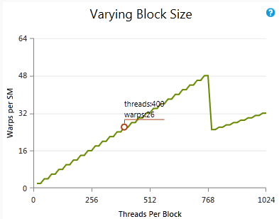
How varying the block size while holding other parameters constant would affect the theoretical Warp occupancy.
How varying the block size while holding other parameters constant would affect the theoretical Warp occupancy. Image: docs.nvidia.com

4. CUDA Cores

4.1 Role of CUDA Cores

CUDA cores, also called SPs (Streaming Processors), are the smallest execution units. Each core executes a single thread from a warp, performing basic arithmetic and logic operations.

4.2 Arithmetic Logic Units (ALUs)

Each CUDA core consists of:

  • FP32 FPU (Floating Point Unit)
  • INT ALU (Integer Arithmetic Unit)
  • Optional support for FP64, depending on SM design

4.3 SIMD Execution under SIMT Model

NVIDIA employs a SIMT (Single Instruction, Multiple Thread) model. Each warp executes one instruction at a time across 32 CUDA cores. Despite the SIMT term, the execution model is close to SIMD, with divergence managed by disabling inactive lanes.

4.4 Register Files and Local Storage

Each thread gets a set of registers from the SM’s register file. Efficient register usage is critical to avoiding spills to slower local memory.


5. Specialized Units within SMs

5.1 Tensor Cores

Tensor cores are designed to accelerate matrix multiplications—key in deep learning. They support:

  • FP16, TF32, INT8, and FP4 (in Blackwell)
  • Mixed-precision compute
  • Fused Multiply-Add (FMA) operations on tiles of 4×4, 8×8 matrices

5.2 Special Function Units (SFUs)

SFUs compute transcendental functions like sine, cosine, exp, log, and square root. These are not time-critical in AI workloads but crucial in graphics.

5.3 Load/Store Units (LSUs)

LSUs manage memory operations between registers, shared memory, and L1/L2 caches. Optimizing memory throughput requires understanding how LSUs queue and coalesce memory transactions.


6. Summary and Practical Takeaways

Understanding the hierarchical breakdown of GPC → TPC → SM → CUDA core helps:

  • Optimize kernel launch configurations
  • Maximize warp occupancy
  • Minimize divergence and memory stalls
  • Align workloads with hardware capabilities

In the next part of the series, we’ll explore Tensor Cores and RT Cores in-depth—covering how NVIDIA has fused graphics and AI acceleration into a unified pipeline.

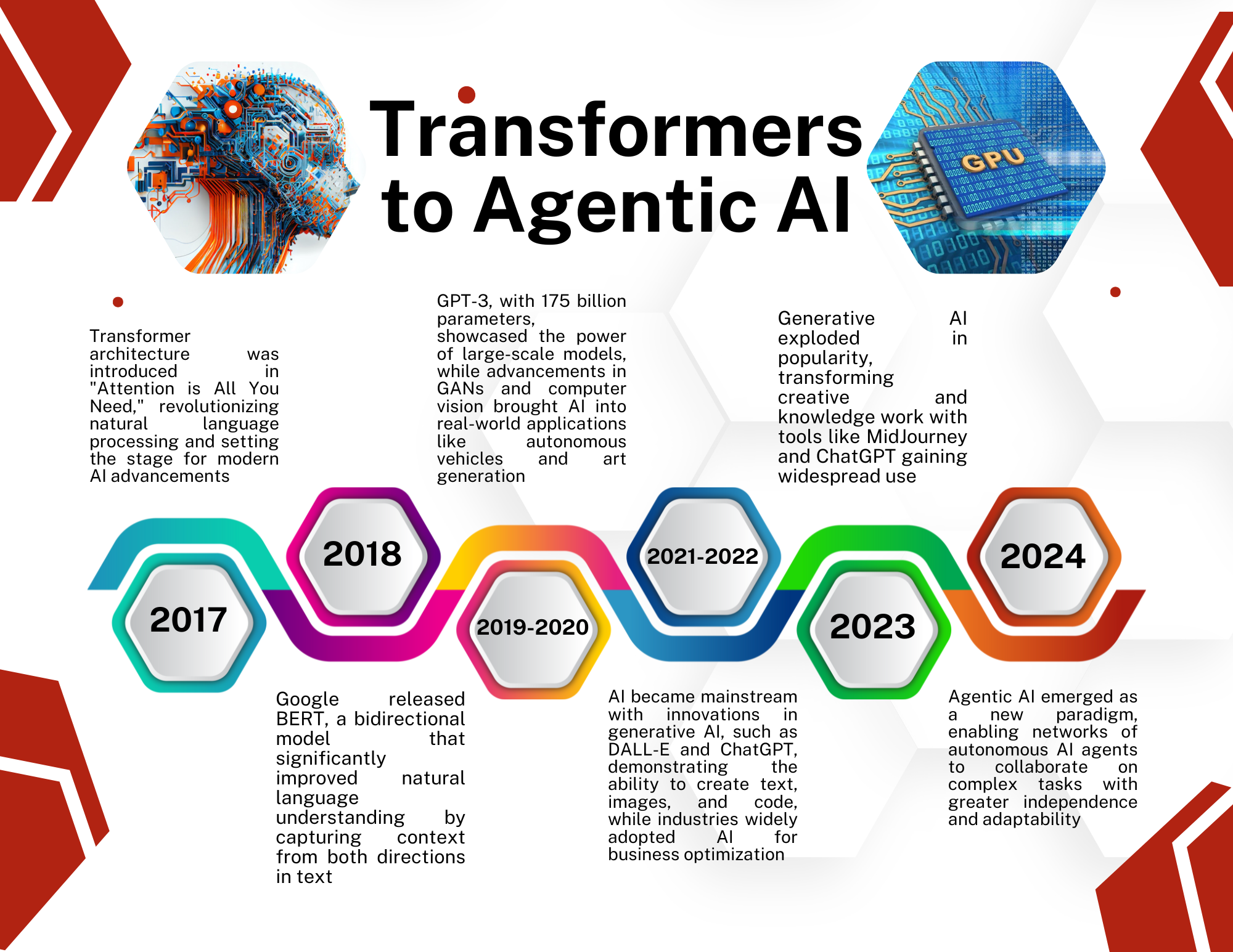
Timeline from Transformers to LLMs and Agentic AI

Since the groundbreaking 2017 paper “Attention is All You Need” introduced the Transformer architecture, the field of artificial intelligence has undergone a rapid and transformative evolution. This blog post will explore the chronology of important events that have shaped the AI landscape, leading up to the current era of Large Language Models (LLMs) and agentic AI. Let us visit the timeline from Transformers to LLM and Agentic AI

2017: The Transformer Revolution

The journey begins with the publication of “Attention is All You Need” by Google scientists in 2017. This paper introduced the Transformer architecture, which relied solely on attention mechanisms, dispensing with recurrence and convolutions entirely. The new model demonstrated superior translation quality and efficiency in machine translation tasks, setting the stage for a paradigm shift in natural language processing.

2018: BERT and the Rise of Bidirectional Models

Building on the success of Transformers, 2018 saw the introduction of BERT (Bidirectional Encoder Representations from Transformers) by Google researchers. BERT’s innovation lay in its bidirectional nature, allowing it to capture context from both directions in text data. This breakthrough significantly improved performance across various language tasks, from question-answering to sentiment analysis.

2019-2020: The GPT Era Begins

OpenAI’s release of GPT-3 (Generative Pre-trained Transformer 3) in 2020 marked a significant milestone in the development of large language models. With 175 billion parameters, GPT-3 demonstrated unprecedented capabilities in natural language understanding and generation, capturing the imagination of researchers and the public alike.

2021-2022: AI Goes Mainstream

During this period, AI technologies began to permeate various industries and applications:

  • AI in Healthcare: The healthcare and pharmaceutical sectors emerged as early adopters of AI, leveraging it for tasks such as appointment scheduling, patient care, and personalized treatment.
  • Self-Driving Vehicles: AI agents moved beyond software into the physical world, making real-time, high-stakes decisions in autonomous vehicles.
  • Code Generation: AI systems like GitHub Copilot began assisting developers in writing code, hinting at the potential for AI to transform software development.
Timeline from Transformers to LLM and Agentic AI

2023: The Year of Generative AI

2023 saw an explosion in generative AI applications, with tools like DALL-E, Midjourney, and ChatGPT capturing public attention. These models demonstrated the ability to generate high-quality text, images, and even code, sparking discussions about the future of creative work and knowledge work.

2024: The Dawn of Agentic AI

As we moved into 2024, the concept of Agentic AI began to take shape. This new paradigm represented a shift from isolated AI tasks to specialized, interconnected agents capable of more autonomous operation. Key developments included:

  • Multi-Agent Systems: AI agents began working collaboratively to solve complex problems, simulating human teamwork in digital environments.
  • Small Language Models (SLMs): The adoption of SLMs alongside LLMs offered new possibilities for efficient, task-specific AI solutions.
  • AI Orchestration: Frameworks for coordinating multiple AI agents emerged, allowing for more complex problem-solving approaches.

2025: The Year of Agentic AI

As we stand in 2025, Agentic AI has become the new frontier in artificial intelligence. This evolution is characterized by several key trends:

  1. Autonomous Decision-Making: AI agents now operate with greater independence, capable of long-term planning and adapting to changing conditions without constant human oversight.
  2. AI Engineers: Systems like Devin AI are now capable of debugging and writing code on their own, pushing the boundaries of what AI can achieve in software development.
  3. Industry Transformation: Agentic AI is revolutionizing various sectors, with the potential to take over entire departments in organizations. For example:
    • In healthcare, AI agents manage tasks from appointment scheduling to personalized treatment plans.
    • In customer service, AI-driven virtual assistants provide increasingly sophisticated and personalized support.
  4. Multi-Agent Collaboration: OpenAI’s introduction of “Swarm,” an experimental framework for coordinating networks of AI agents, has opened new possibilities for complex problem-solving.
  5. Enhanced Personalization: Advanced learning algorithms enable AI agents to tailor services and products to individual needs, creating highly personalized experiences across industries.
  6. Scalable Automation: AI agents are driving automation at an unprecedented scale, from small businesses to large enterprises, significantly reducing costs and operational inefficiencies.
  7. Continuous Learning and Adaptation: Agentic AI systems demonstrate the ability to learn autonomously and adapt to dynamic environments, enabling faster growth and efficiency across sectors.

As we look to the future, the potential of Agentic AI seems boundless. From enhancing decision-making processes to revolutionizing entire industries, these intelligent agents are poised to transform the way we work, create, and solve problems. However, this rapid advancement also brings new challenges in ethics, privacy, and workforce adaptation that society must address.

We saw and have actually lived through this timeline from Transformers to LLM and Agentic AI. The journey has been remarkably swift, showcasing the exponential pace of innovation in artificial intelligence. As we explore the vast potential of Agentic AI, the broader quest for Artificial General Intelligence (AGI) remains a captivating goal. AGI aims to create intelligent systems capable of performing any intellectual task that humans can and represents the ultimate frontier in artificial intelligence. Another interesting article on this topic can be found here. For a deeper dive into the most basic concepts on AI and Machine Learning please visit my other blog pages.

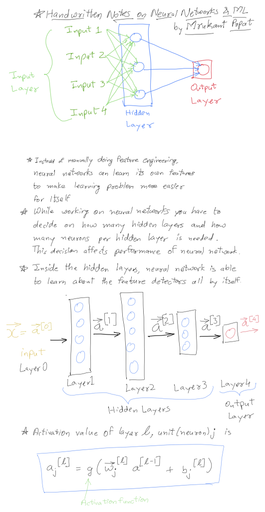
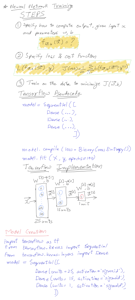
Hand written notes on Neural Networks and ML course by Andrew Ng

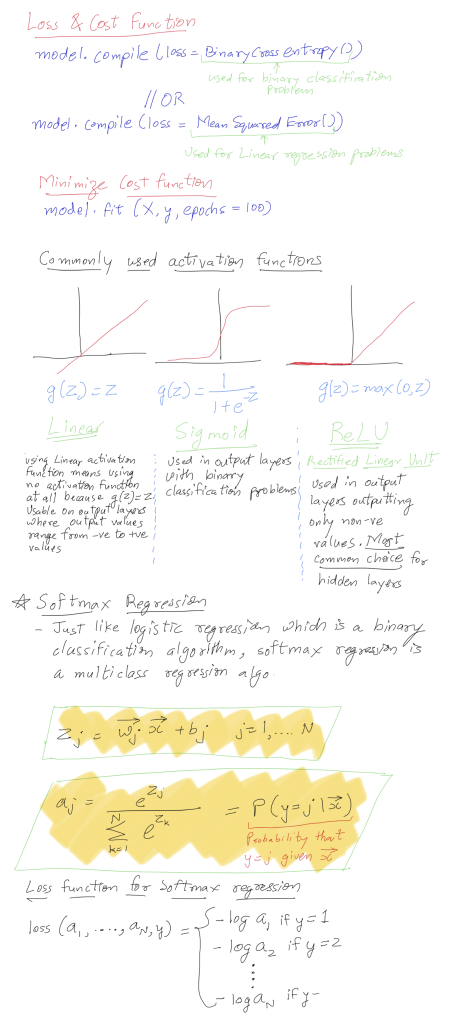
About 2018 when I started working on Machine learning I took many courses. Here are my hand written notes on Neural Networks and ML course by Andrew Ng. It focuses on the fundamental concepts covered in the course, including Logistic Regression, Neural Networks, and Softmax Regression. Buckle up for some equations and diagrams!

Part 1: Logistic Regression – The Binary Classification Workhorse

Logistic regression reigns supreme for tasks where the target variable (y) can only take on two distinct values, typically denoted as 0 or 1. It essentially calculates the probability (a) of y belonging to class 1, given a set of input features (x). Here’s a breakdown of the process:

  1. Linear Combination: The model calculates a linear score (z) by taking a weighted sum of the input features (x) and their corresponding weights (w). We can represent this mathematically as:

    z = w_1x_1 + w_2x_2 + … + w_nx_n

    (where n is the number of features)
  2. Sigmoid Function: This linear score (z) doesn’t directly translate to a probability. The sigmoid function (σ) steps in to transform this score into a value between 0 and 1, representing the probability (a) of y belonging to class 1. The sigmoid function is typically defined as:

a = \sigma(z) = \frac{1}{1 + e^{-z}}

Sigmoid Function Plot / Logistic Curve


Key takeaway: 1 – a represents the probability of y belonging to class 0. This is because the sum of probabilities for both classes must always equal 1.

Part 2: Demystifying Neural Networks – Building Blocks and Forward Propagation

  1. Perceptrons – The Basic Unit: Neural networks are built using perceptrons, the fundamental unit inspired by biological neurons. A perceptron takes weighted inputs (just like logistic regression), performs a linear transformation, and applies an activation function to generate an output.
  2. Activation Functions: While sigmoid functions are common in logistic regression and the initial layers of neural networks, other activation functions like ReLU (Rectified Linear Unit) can also be employed. These functions introduce non-linearity, allowing the network to learn more complex patterns in the data.
  3. Layering Perceptrons: Neural networks are not limited to single perceptrons. We can stack multiple perceptrons into layers, where each neuron in a layer receives outputs from all the neurons in the previous layer. This creates a complex network of interconnected units.
  4. Forward Propagation: Information flows through the network in a forward direction, layer by layer. In each layer, the weighted sum of the previous layer’s outputs is calculated and passed through an activation function. This process continues until the final output layer produces the network’s prediction.

Part 3: Unveiling Backpropagation – The Learning Algorithm

But how do these neural networks actually learn? Backpropagation is the hero behind the scenes! It allows the network to adjust its weights and biases in an iterative manner to minimize the error between the predicted and actual outputs.

  1. Cost Function: We define a cost function that measures how well the network’s predictions align with the actual labels. A common cost function for classification problems is the cross-entropy loss.
  2. Error Calculation: Backpropagation calculates the error (difference between prediction and actual value) at the output layer and propagates it backward through the network.
  3. Weight and Bias Updates: Based on the calculated errors, the weights and biases of each neuron are adjusted in a way that minimizes the overall cost function. This process is repeated iteratively over multiple training epochs until the network converges to a minimum error state.

Part 4: Softmax Regression – Expanding Logistic Regression for Multi-Class Classification

Logistic regression excels in binary classification, but what happens when we have more than two possible class labels for the target variable (y)? Softmax regression emerges as a powerful solution!

  1. Generalizing Logistic Regression: Softmax regression can be viewed as an extension of logistic regression for multi-class problems. It calculates a set of class scores (z_i) for each possible class (i).
  2. The Softmax Function: Similar to the sigmoid function, softmax takes these class scores (z_i) and transforms them into class probabilities (a_i) using the following formula:

a_i = \frac{e^{z_i}}{\sum\limits_{j=1}^{C} e^{z_j}}

(where Σ represents the sum over all possible classes j)
Key takeaway: This function ensures that all the class probabilities (a_i) sum up to 1, which is a crucial requirement for a valid probability distribution. Intuitively, for a given input (x), only one class can be true, and the softmax function effectively distributes the probability mass across all classes based on their corresponding z_i scores.

Softmax Function Curve

  1. Interpretation of Class Probabilities: Each class probability (a_i) represents the model’s estimated probability of the target variable (y) belonging to class i, given the input features (x). This probabilistic interpretation empowers us to not only predict the most likely class but also gauge the model’s confidence in that prediction.

Part 5: Putting It All Together – Training and Cost Function for Softmax Regression

Part 5: Putting It All Together – Training and Cost Function for Softmax Regression

While we’ve focused on the mechanics of softmax, training a softmax regression model involves a cost function. Here’s a brief overview:

  1. Negative Log-Likelihood Cost Function: Softmax regression typically employs the negative log-likelihood cost function. This function penalizes the model for assigning low probabilities to the correct class and vice versa. Mathematically, the cost function can be represented as:Cost=−Σ(yi∗log(ai))
    (where y_i is 1 for the correct class and 0 otherwise)
  2. Model Optimization: During training, the model aims to minimize this cost function by adjusting its weights and biases through backpropagation. As the cost function decreases, the model learns to produce class probabilities that better reflect the underlying data distribution.

Conclusion: A Stepping Stone to Deep Learning

These blog and hand written notes on Neural Networks and ML has provided a condensed yet detailed exploration of logistic regression, neural networks, and softmax regression, concepts covered in Andrew Ng’s Advanced Learning Algorithms course. Understanding these fundamental building blocks equips you to delve deeper into the fascinating world of Deep Learning and explore more advanced architectures like Convolutional Neural Networks (CNNs) and Recurrent Neural Networks (RNNs).Remember, this is just the beginning of your Deep Learning journey!

I hope these detailed hand written notes on Neural Networks and ML with diagrams prove helpful for your Deep Learning studies!