Tag: logistic regression

About 2018 when I started working on Machine learning I took many courses. Here are my hand written notes on Neural Networks and ML course by Andrew Ng. It focuses on the fundamental concepts covered in the course, including Logistic Regression, Neural Networks, and Softmax Regression. Buckle up for some equations and diagrams!

Part 1: Logistic Regression – The Binary Classification Workhorse

Logistic regression reigns supreme for tasks where the target variable (y) can only take on two distinct values, typically denoted as 0 or 1. It essentially calculates the probability (a) of y belonging to class 1, given a set of input features (x). Here’s a breakdown of the process:

1. Linear Combination: The model calculates a linear score (z) by taking a weighted sum of the input features (x) and their corresponding weights (w). We can represent this mathematically as:
   
   z = w_1x_1 + w_2x_2 + … + w_nx_n
   
   (where n is the number of features)
2. Sigmoid Function: This linear score (z) doesn’t directly translate to a probability. The sigmoid function (σ) steps in to transform this score into a value between 0 and 1, representing the probability (a) of y belonging to class 1. The sigmoid function is typically defined as:

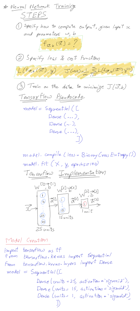
Part 2: Demystifying Neural Networks – Building Blocks and Forward Propagation

1. Perceptrons – The Basic Unit: Neural networks are built using perceptrons, the fundamental unit inspired by biological neurons. A perceptron takes weighted inputs (just like logistic regression), performs a linear transformation, and applies an activation function to generate an output.
2. Activation Functions: While sigmoid functions are common in logistic regression and the initial layers of neural networks, other activation functions like ReLU (Rectified Linear Unit) can also be employed. These functions introduce non-linearity, allowing the network to learn more complex patterns in the data.
3. Layering Perceptrons: Neural networks are not limited to single perceptrons. We can stack multiple perceptrons into layers, where each neuron in a layer receives outputs from all the neurons in the previous layer. This creates a complex network of interconnected units.
4. Forward Propagation: Information flows through the network in a forward direction, layer by layer. In each layer, the weighted sum of the previous layer’s outputs is calculated and passed through an activation function. This process continues until the final output layer produces the network’s prediction.

Part 3: Unveiling Backpropagation – The Learning Algorithm

But how do these neural networks actually learn? Backpropagation is the hero behind the scenes! It allows the network to adjust its weights and biases in an iterative manner to minimize the error between the predicted and actual outputs.

1. Cost Function: We define a cost function that measures how well the network’s predictions align with the actual labels. A common cost function for classification problems is the cross-entropy loss.
2. Error Calculation: Backpropagation calculates the error (difference between prediction and actual value) at the output layer and propagates it backward through the network.
3. Weight and Bias Updates: Based on the calculated errors, the weights and biases of each neuron are adjusted in a way that minimizes the overall cost function. This process is repeated iteratively over multiple training epochs until the network converges to a minimum error state.

Part 4: Softmax Regression – Expanding Logistic Regression for Multi-Class Classification

Logistic regression excels in binary classification, but what happens when we have more than two possible class labels for the target variable (y)? Softmax regression emerges as a powerful solution!

1. Generalizing Logistic Regression: Softmax regression can be viewed as an extension of logistic regression for multi-class problems. It calculates a set of class scores (z_i) for each possible class (i).
2. The Softmax Function: Similar to the sigmoid function, softmax takes these class scores (z_i) and transforms them into class probabilities (a_i) using the following formula:

(where Σ represents the sum over all possible classes j)
Key takeaway: This function ensures that all the class probabilities (a_i) sum up to 1, which is a crucial requirement for a valid probability distribution. Intuitively, for a given input (x), only one class can be true, and the softmax function effectively distributes the probability mass across all classes based on their corresponding z_i scores.

Softmax Function Curve

3. Interpretation of Class Probabilities: Each class probability (a_i) represents the model’s estimated probability of the target variable (y) belonging to class i, given the input features (x). This probabilistic interpretation empowers us to not only predict the most likely class but also gauge the model’s confidence in that prediction.

Part 5: Putting It All Together – Training and Cost Function for Softmax Regression

Part 5: Putting It All Together – Training and Cost Function for Softmax Regression

While we’ve focused on the mechanics of softmax, training a softmax regression model involves a cost function. Here’s a brief overview:

1. Negative Log-Likelihood Cost Function: Softmax regression typically employs the negative log-likelihood cost function. This function penalizes the model for assigning low probabilities to the correct class and vice versa. Mathematically, the cost function can be represented as:Cost=−Σ(yi∗log(ai))
   (where y_i is 1 for the correct class and 0 otherwise)
   
2. Model Optimization: During training, the model aims to minimize this cost function by adjusting its weights and biases through backpropagation. As the cost function decreases, the model learns to produce class probabilities that better reflect the underlying data distribution.

Conclusion: A Stepping Stone to Deep Learning

These blog and hand written notes on Neural Networks and ML has provided a condensed yet detailed exploration of logistic regression, neural networks, and softmax regression, concepts covered in Andrew Ng’s Advanced Learning Algorithms course. Understanding these fundamental building blocks equips you to delve deeper into the fascinating world of Deep Learning and explore more advanced architectures like Convolutional Neural Networks (CNNs) and Recurrent Neural Networks (RNNs).Remember, this is just the beginning of your Deep Learning journey!

I hope these detailed hand written notes on Neural Networks and ML with diagrams prove helpful for your Deep Learning studies!