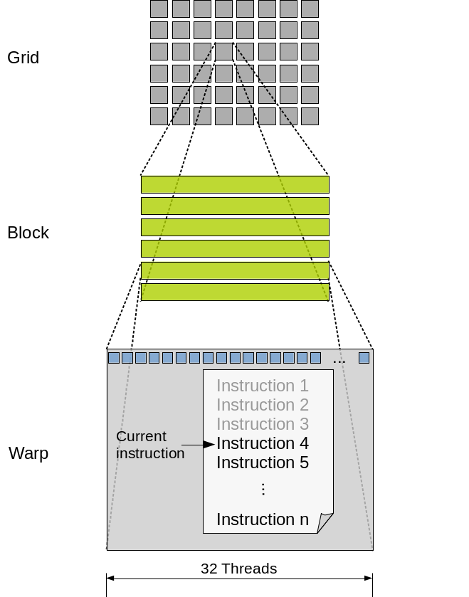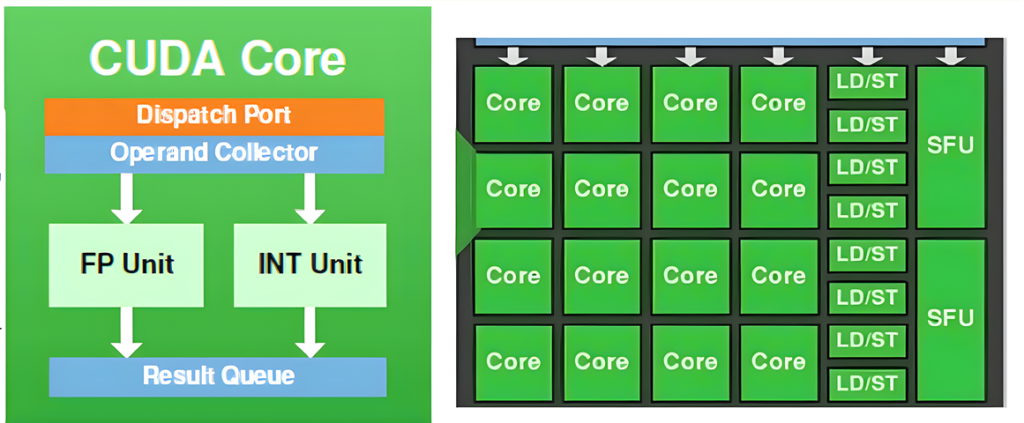
This blog is Part 3 in our Nvidia GPU blog series. In Parts 1 and 2, we explored the fundamentals of NVIDIA GPU architecture: from CUDA cores to streaming multiprocessors (SMs) and warp schedulers. Today, we transition into what sets modern NVIDIA GPUs apart-the Tensor Cores and Ray Tracing (RT) Cores-two hardware innovations that fuel cutting-edge advancements in AI computation and real-time rendering.
NVIDIA Tensor and Ray Tracing Cores have revolutionized , making GPUs the backbone of deep learning workloads. Meanwhile, RT Cores enabled real-time photorealistic graphics, redefining visual realism in games and simulations. In this post, we dissect their architectures, working principles, and how they seamlessly integrate into the GPU pipeline.
🧠 Tensor Cores – Unleashing AI Performance
Architectural Evolution and Integration
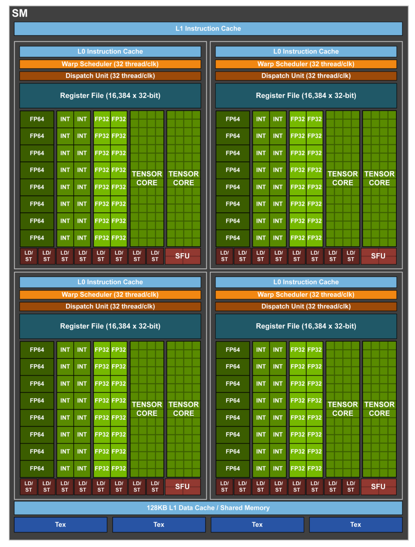
Tensor Cores were introduced in the Volta (GV100) architecture, setting a new benchmark for AI acceleration. Each Streaming Multiprocessor (SM) houses multiple Tensor Cores, tightly coupled with CUDA cores and other functional units. This co-location allows Tensor Cores to offload matrix-heavy operations like convolutions and fully connected layers, while CUDA cores handle scalar/vector instructions.
Across architectures:
- Volta: First appearance; FP16 precision support.
- Turing: Added INT8 & INT4 precision for inference workloads.
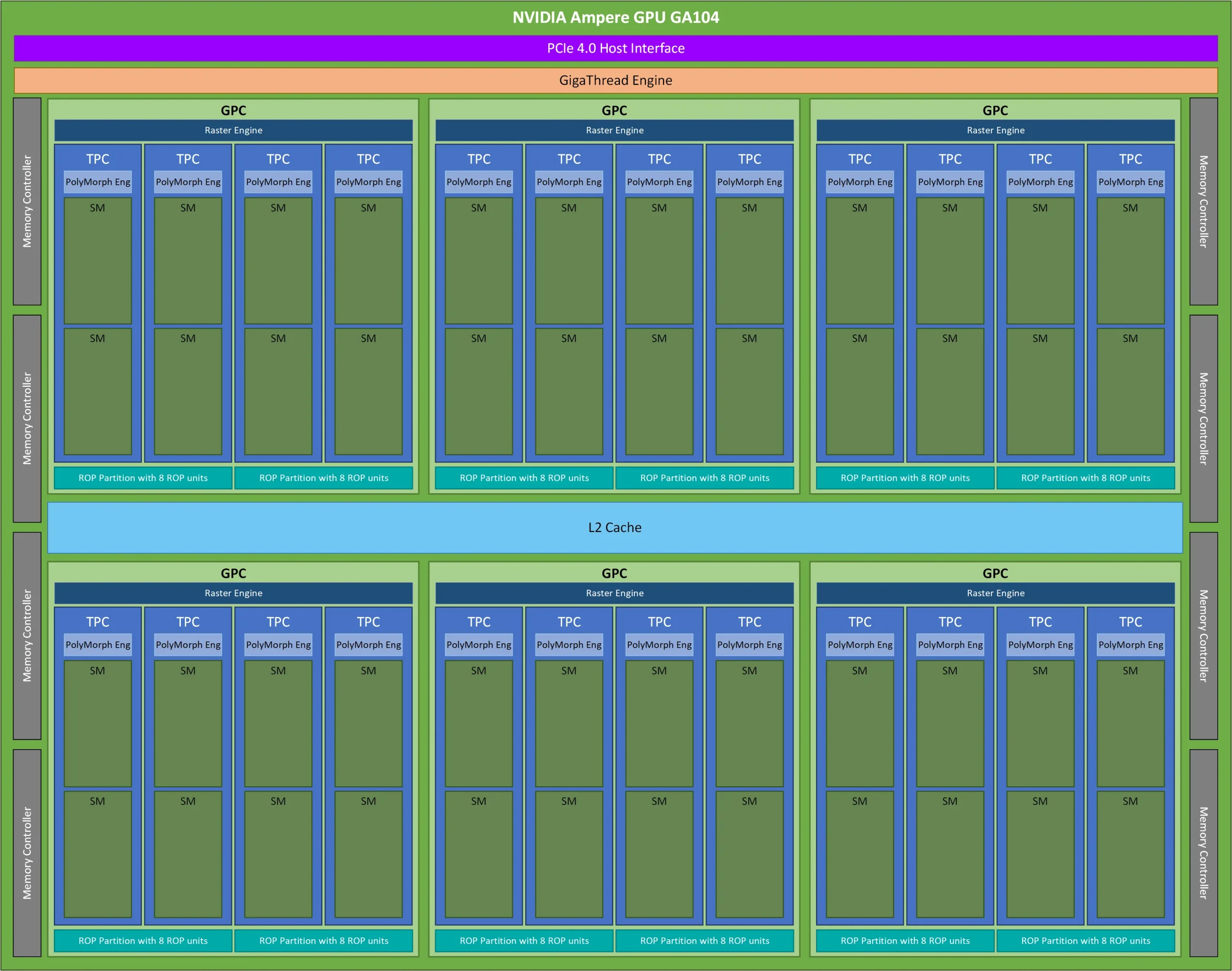
- Ampere: Introduced TF32 and enhanced sparsity support.
- Hopper: Revolutionized with FP8 and the Transformer Engine.
Each SM includes hardware schedulers that coordinate the execution of Tensor Core operations alongside traditional CUDA threads, ensuring maximal occupancy and throughput.
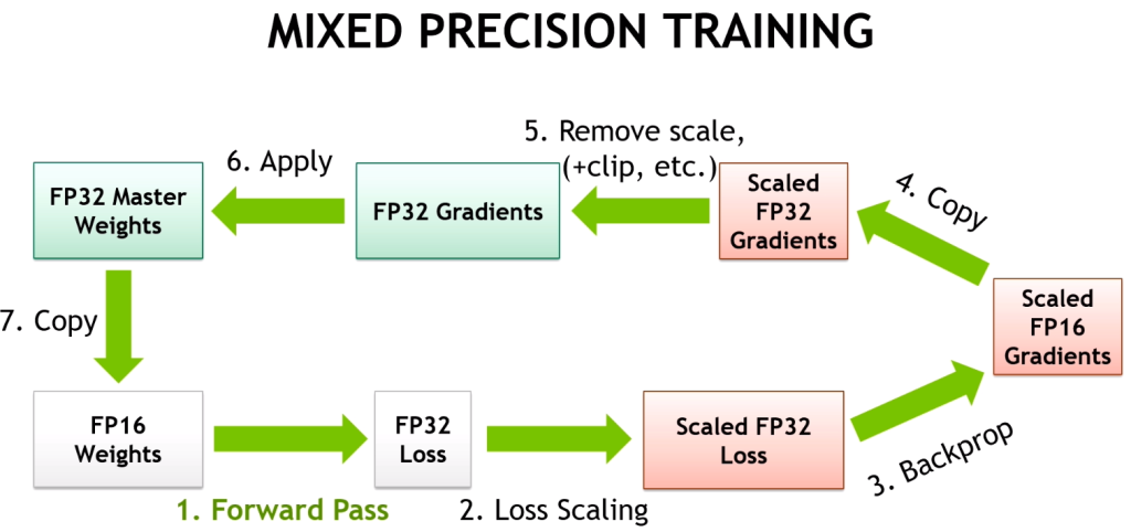
Precision Modes: FP32, FP16, TF32, INT8, FP8, and FP4
Precision is critical in balancing performance and numerical stability.
- FP32: Full precision; used in scientific computing.
- TF32: Ampere’s innovation, offering FP32 dynamic range but with FP16 compute efficiency-achieves up to 10× speedup in deep learning training.
- FP16 (Half Precision): Ideal for neural nets tolerant to low precision; critical in deep learning inference.
- INT8 & INT4: Efficient for low-latency inference, especially on edge devices.
- FP8 & FP4: Next-gen precision; FP8 is central to Hopper’s Transformer Engine, while FP4 is emerging for ultra-low-power inference.
Tensor Cores dynamically downscale or upscale precision based on kernel requirements, facilitated by NVIDIA’s cuDNN and TensorRT libraries.
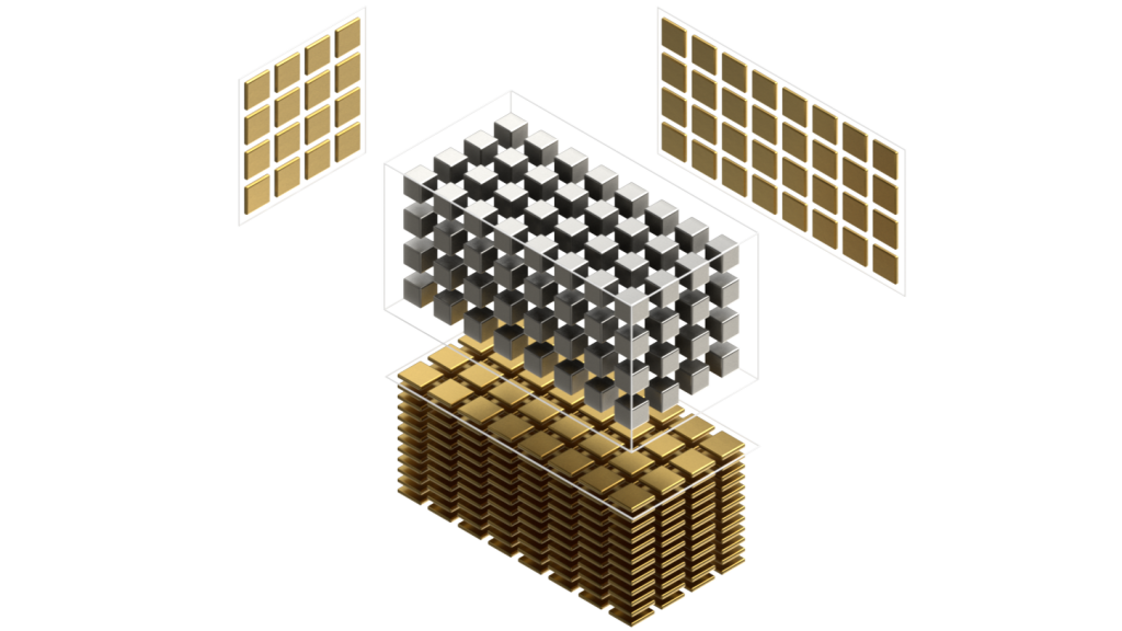
In-Depth: Matrix Multiply-Accumulate (MMA) Engine
At the heart of Tensor Cores is the Matrix Multiply-Accumulate (MMA) Engine. The MMA pipeline is designed to perform:
D=A×B+C
For matrix tiles (commonly 16×16). The Tensor Core parallelizes these tiles across multiple hardware lanes, enabling:
- 16×16×16 FP16 MMAs in a single cycle (Volta-Ampere).
- Dynamic 8×8 tiles with FP8 in Hopper for optimized attention layers.
Tensor Cores rely on warp-level primitives, where threads in a warp collaborate on MMA operations. NVIDIA’s CUDA WMMA API provides direct access to these functionalities.
Transformer Engine & Sparsity Acceleration
Transformer models-which power LLMs like GPT-have unique computational patterns. Hopper’s Transformer Engine:
- Detects per-layer precision requirements (FP16 vs FP8).
- Dynamically adjusts execution precision at runtime.
- Leverages context-aware sparsity, which identifies zero-value weights and skips redundant computation.
This enables 50%+ reductions in compute/memory without sacrificing accuracy. Ampere introduced 4:2 structured sparsity, doubling throughput for sparse models.
🎮 Ray Tracing Cores – Enabling Cinematic Real-Time Ray Tracing
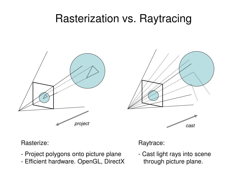
The Shift from Rasterization to Path Tracing
Rasterization dominates traditional graphics pipelines by projecting 3D geometry into 2D fragments. However, it fails to simulate true light behavior like global illumination and caustics. Ray tracing simulates:
- Primary rays (camera → scene)
- Reflection/refraction rays (mirror/glass)
- Shadow rays (light occlusion)
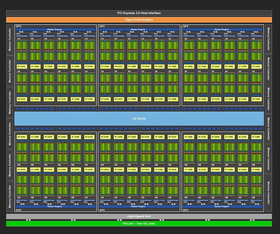
RT Cores were introduced in Turing, transforming ray tracing from a batch process to a real-time application.
BVH Traversal and Intersection Hardware
The core of RT Core acceleration lies in BVH (Bounding Volume Hierarchy) traversal.
- BVH Tree: Scene geometry is hierarchically partitioned into boxes.
- Traversal: RT Cores quickly determine if rays intersect bounding boxes-rejecting entire regions early.
Once inside a leaf node, Ray-Triangle Intersection units calculate precise hit points using barycentric coordinates and optimized hardware pipelines.
Performance: RTX 3090 achieves 10 billion BVH tests/sec, enabling complex environments at playable frame rates.
Multi-Stage Ray Shading Pipeline
The shading pipeline includes:
- Ray Generation Shader: Initiates rays.
- Closest Hit Shader: Determines material/shader logic on hit.
- Any Hit Shader: Early exits for transparency effects.
- Miss Shader: Background/environment mapping.
Each ray potentially spawns secondary rays, making recursive traversal necessary. Tensor Cores assist by AI-denoising noisy samples-enhancing visual quality without full sampling.
🤝 Tensor + RT: DLSS and Hybrid Workloads
DLSS (Deep Learning Super Sampling) epitomizes the synergy of Tensor + RT Cores. The workflow:
- RT Cores: Render base frame (lower resolution).
- Tensor Cores: Upscale + reconstruct via AI models.
DLSS 3.0 (Ada Lovelace) even predicts in-between frames using motion vectors + optical flow estimation-massively boosting FPS in ray-traced environments.
This hybrid method achieves 4K quality at 1080p costs, revolutionizing graphics performance.
🧪 Developer Toolkit: Leveraging Tensor & RT Cores
For AI:
- CUDA WMMA API
- cuBLAS/cuDNN
- TensorRT
For Graphics:
- Vulkan/DXR
- NVIDIA OptiX
- Nsight Visual Profiler
Profiling tools allow warp-occupancy tracking, Tensor Core utilization, and RT core tracing, helping developers fine-tune performance.
📈 Conclusion
NVIDIA’s Tensor and Ray Tracing Cores are cornerstones of modern GPU architecture, unlocking unprecedented capabilities across AI, graphics, and simulation. These specialized cores complement general CUDA compute, enabling applications that were infeasible a decade ago.
In Part 4, we’ll unravel the mysteries of GPU memory subsystems, cache hierarchies, and NVLink/NVSwitch-crucial for multi-GPU scaling.