Deep Dive into GPU Compute Hierarchy

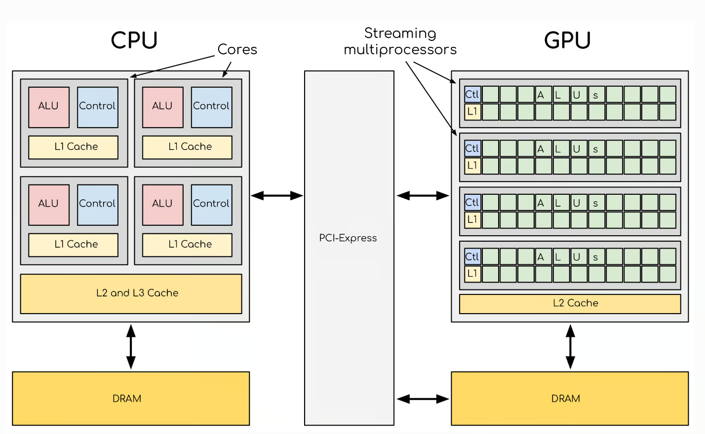
Modern NVIDIA GPUs are feats of hierarchical design, optimized to maximize parallelism, minimize latency, and deliver staggering computational throughput. Building upon Part 1, which introduced the high-level architecture of NVIDIA GPUs, this is Part2 – a Deep dive into GPU Compute Hierarchy: Graphics Processing Clusters (GPCs), Texture Processing Clusters (TPCs), Streaming Multiprocessors (SMs), and CUDA cores. Understanding this hierarchy is essential for anyone looking to write optimized CUDA code or analyze GPU-level performance.


1. Graphics Processing Clusters (GPCs)

1.1 Overview

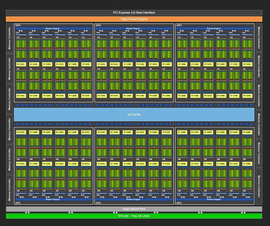
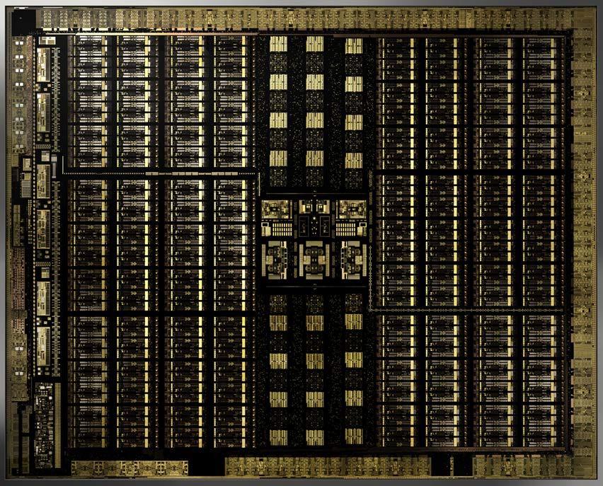
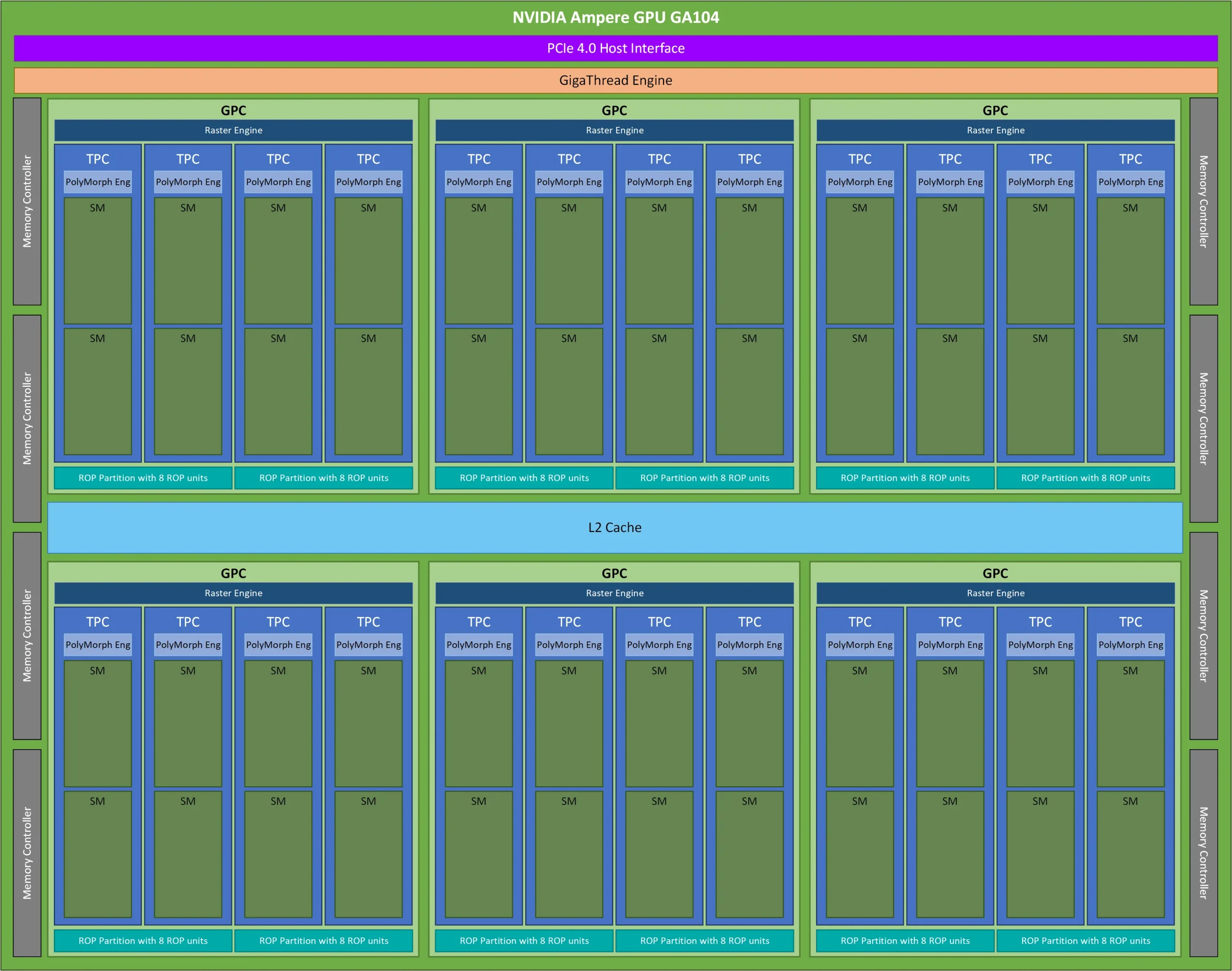
At the top of NVIDIA’s compute hierarchy lies the Graphics Processing Cluster. A GPC is an independently operating unit within the GPU, responsible for distributing workloads efficiently across its internal resources. Each GPC contains a set of Texture Processing Clusters (TPCs), Raster Engines, and shared control logic.

📊 GPC Block Diagram:

Nvidia Turing TU102 Full GPU with 72 SM Units.
Nvidia Turing TU102 Full GPU with 72 SM Units. Image : developer.nvidia.com
Internal Die layout of Nvida Turing TU102 GPU .
Internal Die layout of Nvida Turing TU102 GPU . Image : developer.nvidia.com

1.2 GPC Architecture

Each GPC includes:

  • One or more Raster Engines
  • Several TPCs (typically 2 to 8 depending on the GPU tier)
  • A Geometry Engine (in graphics workloads)

📘 Example GPC layout in RTX 30 series:

Nvidia RTX30 GPC block Diagram
Nvidia RTX30 GPC block Diagram. Image: Nvidia Ampere GA102 GPU Architecture document

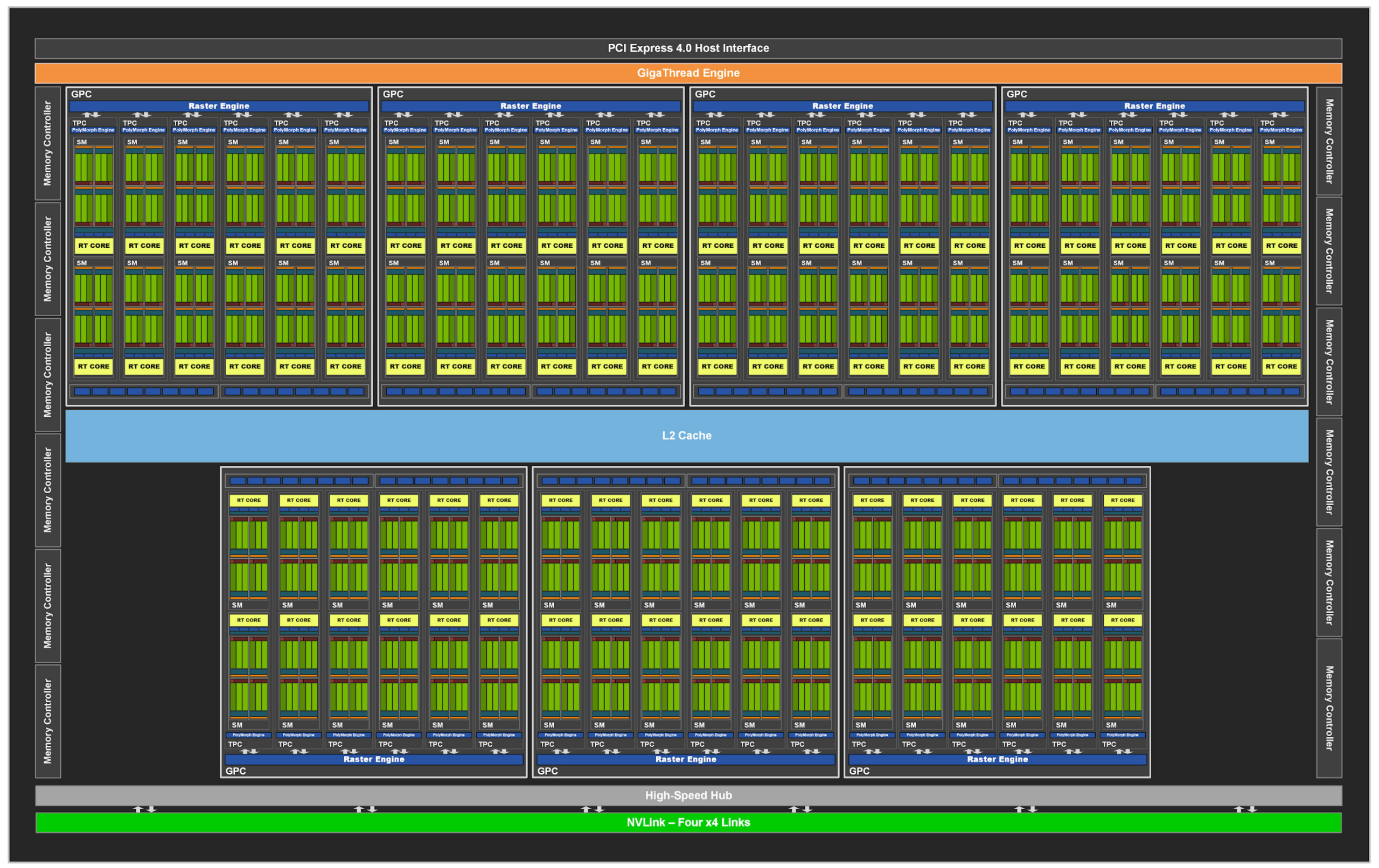
1.3 Scalability Role

More GPCs generally equate to more parallel compute and graphics capability. High-end GPUs like the H100 feature many GPCs to support large-scale AI workloads, while mobile GPUs may only include one or two.


2. Texture Processing Clusters (TPCs)

2.1 Role of TPCs

TPCs are the next level down. A TPC groups together Streaming Multiprocessors (SMs) and a set of fixed-function texture units, providing both compute and graphics acceleration. Originally optimized for texture mapping and rasterization, TPCs in modern GPUs support general-purpose compute as well.

2.2 Components of a TPC

Each TPC typically contains:

  • Two Streaming Multiprocessors (SMs)
  • Shared L1 cache
  • Texture units (for graphics and compute shaders)
  • A PolyMorph Engine (responsible for vertex attribute setup and tessellation)

📊 TPC Diagram with SMs and Texture Units:

NVIDIA Ampere GA104 architecture showing GPC, TPC, SM.
NVIDIA Ampere GA104 architecture showing GPC, TPC, SM. Image: wolfadvancedtechnology.com

2.3 Texture Mapping

Texture units in the TPC fetch texels from memory, perform filtering (e.g., bilinear, trilinear), and handle texture addressing. These units have been extended to support texture sampling for compute workloads, such as in scientific visualization.


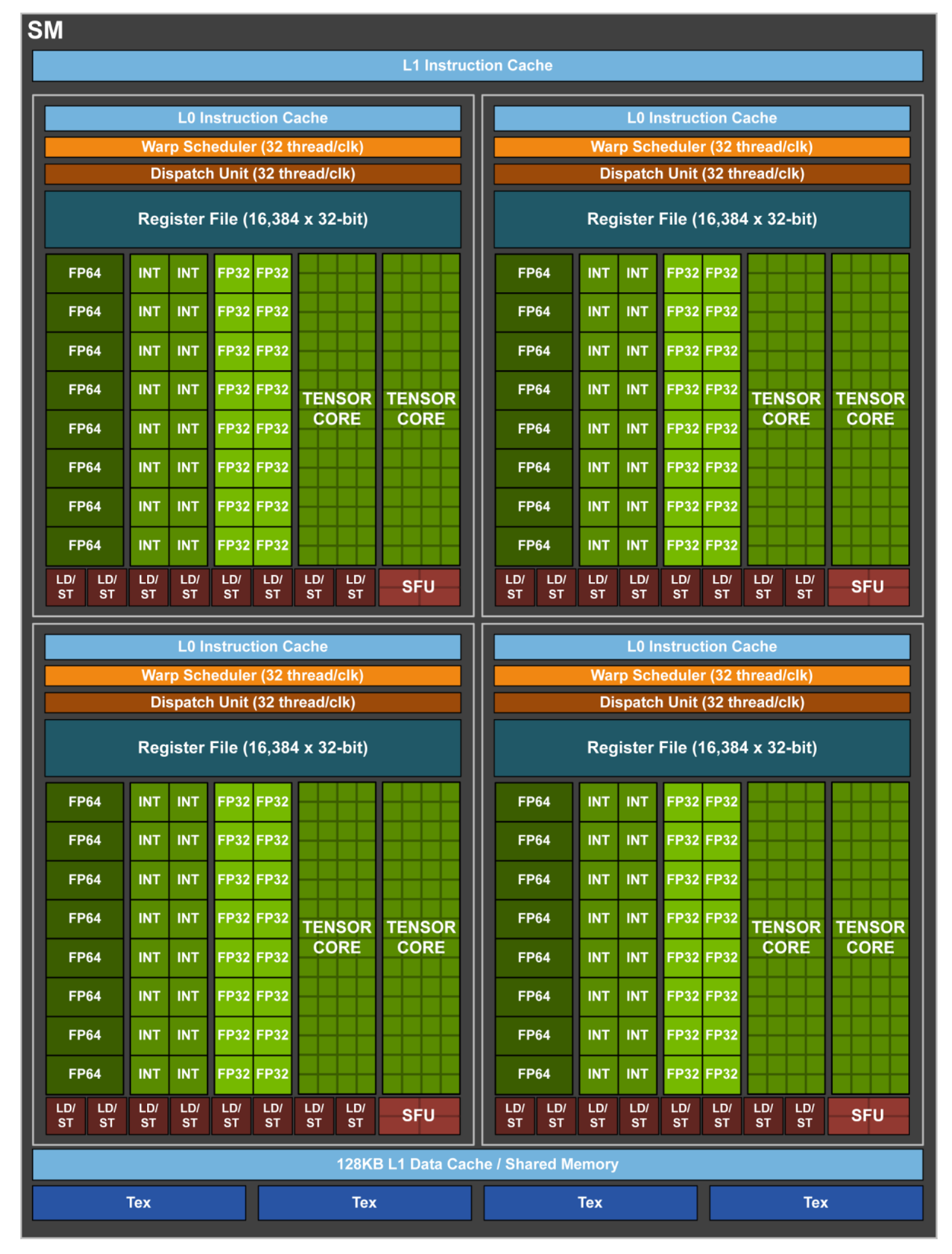
3. Streaming Multiprocessors (SMs)

3.1 Importance of SMs

Streaming Multiprocessors are the core programmable units of NVIDIA GPUs. They execute the majority of instructions, including floating-point arithmetic, integer operations, load/store instructions, and branch logic.

3.2 SM Internal Structure

A modern SM (e.g., in the Hopper H100 or Blackwell B100) consists of:

  • Multiple CUDA cores (up to 128 per SM)
  • Load/Store Units (LSUs)
  • Integer and Floating Point ALUs
  • Tensor Cores (for matrix operations)
  • Special Function Units (SFUs)
  • Warp schedulers and dispatch units
  • Register files
  • Shared memory and L1 cache

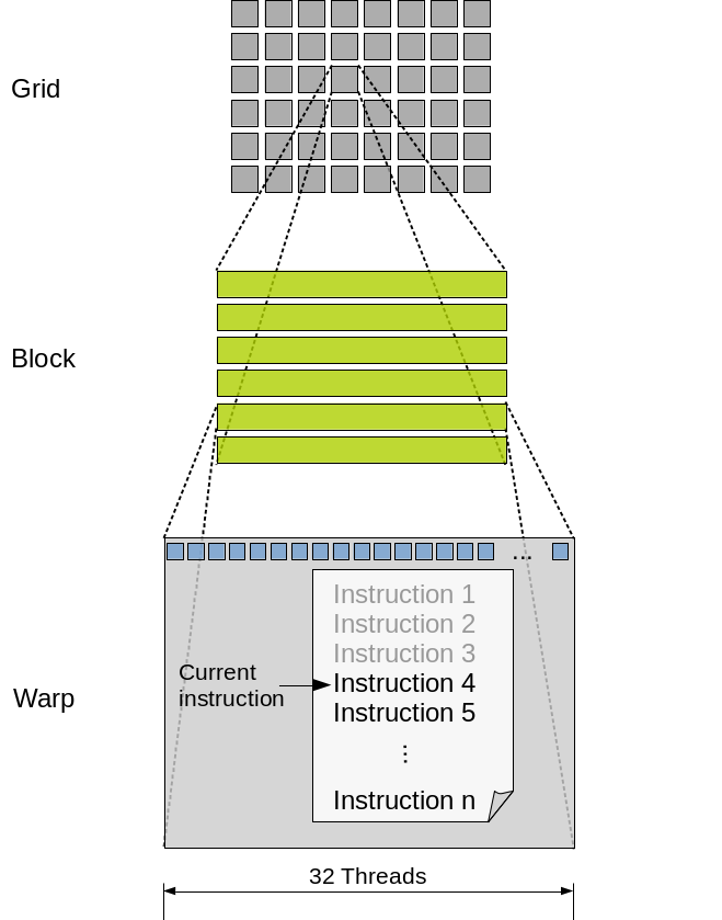
📘 SM Layout Reference (Volta/Hopper SMs):

Nvidia Volta Streaming Multiprovessor (SM) block diagram
Nvidia Volta Streaming Multiprovessor (SM) block diagram. Image: Nvidia Volta Architecture Document

3.3 Warp Scheduling

The warp scheduler picks a ready warp from a warp pool and issues an instruction every clock cycle. Techniques like GTO (Greedy Then Oldest), Round-Robin, or Two-Level scheduling are used.

Key Benefits:

  • Latency hiding: Warps can be swapped out when memory access stalls occur.
  • Concurrency: Independent warps can issue instructions simultaneously.
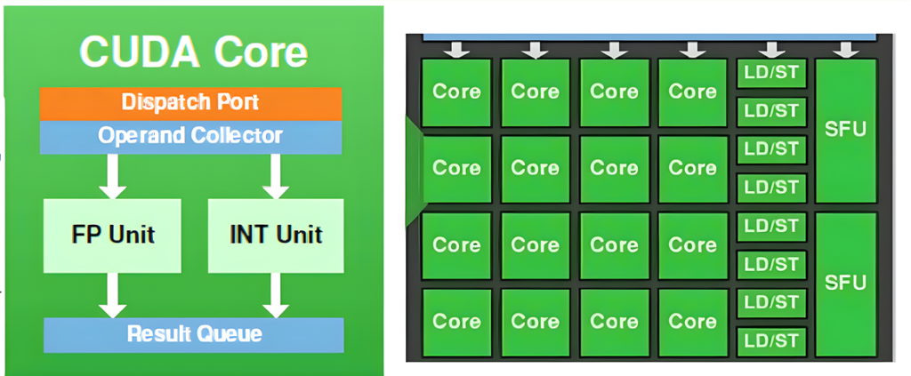
How varying the block size while holding other parameters constant would affect the theoretical Warp occupancy.
How varying the block size while holding other parameters constant would affect the theoretical Warp occupancy. Image: docs.nvidia.com

4. CUDA Cores

4.1 Role of CUDA Cores

CUDA cores, also called SPs (Streaming Processors), are the smallest execution units. Each core executes a single thread from a warp, performing basic arithmetic and logic operations.

4.2 Arithmetic Logic Units (ALUs)

Each CUDA core consists of:

  • FP32 FPU (Floating Point Unit)
  • INT ALU (Integer Arithmetic Unit)
  • Optional support for FP64, depending on SM design

4.3 SIMD Execution under SIMT Model

NVIDIA employs a SIMT (Single Instruction, Multiple Thread) model. Each warp executes one instruction at a time across 32 CUDA cores. Despite the SIMT term, the execution model is close to SIMD, with divergence managed by disabling inactive lanes.

4.4 Register Files and Local Storage

Each thread gets a set of registers from the SM’s register file. Efficient register usage is critical to avoiding spills to slower local memory.


5. Specialized Units within SMs

5.1 Tensor Cores

Tensor cores are designed to accelerate matrix multiplications—key in deep learning. They support:

  • FP16, TF32, INT8, and FP4 (in Blackwell)
  • Mixed-precision compute
  • Fused Multiply-Add (FMA) operations on tiles of 4×4, 8×8 matrices

5.2 Special Function Units (SFUs)

SFUs compute transcendental functions like sine, cosine, exp, log, and square root. These are not time-critical in AI workloads but crucial in graphics.

5.3 Load/Store Units (LSUs)

LSUs manage memory operations between registers, shared memory, and L1/L2 caches. Optimizing memory throughput requires understanding how LSUs queue and coalesce memory transactions.


6. Summary and Practical Takeaways

Understanding the hierarchical breakdown of GPC → TPC → SM → CUDA core helps:

  • Optimize kernel launch configurations
  • Maximize warp occupancy
  • Minimize divergence and memory stalls
  • Align workloads with hardware capabilities

In the next part of the series, we’ll explore Tensor Cores and RT Cores in-depth—covering how NVIDIA has fused graphics and AI acceleration into a unified pipeline.

✅ Introduction to NVIDIA GPU Architecture: Hierarchy, Cores, and Parallelism

👋 Welcome to GPU Architecture 101

In this first post in five-part series, where I introduce you to the NVIDIA GPU architecture—a foundation for parallel computing used in gaming, scientific computing, artificial intelligence, and more.

This guide is designed for engineering students and beginner developers who want to understand how modern GPUs work—from their evolution to core architectural blocks like GPCs, TPCs, SMs, and CUDA Cores.


🧠 What is a GPU and Why Does It Matter?

A GPU (Graphics Processing Unit) is a processor specialized in performing many operations simultaneously. Unlike CPUs, which handle one or a few tasks at a time, GPUs contain thousands of smaller cores to process data in parallel.

A Quick Comparison: GPU vs CPU

Source: Datacamp.com
FeatureCPUGPU
FocusSerial processingParallel processing
Cores4–32 large cores100s–1000s of smaller cores
UsageOS, logic, light appsGraphics, AI, simulations

📊 GPUs are ideal for matrix multiplications, image processing, 3D rendering, and training AI models.


🚀 NVIDIA GPU Architecture Hierarchy

Understanding the hierarchy inside a GPU is key to mastering performance tuning and CUDA programming.

Hernandez Fernandez, Moises & Guerrero, Ginés & Cecilia, José & García, José & Inuggi, Alberto & Jbabdi, Saad & Behrens, Timothy & Sotiropoulos, Stamatios. (2015). Erratum: Accelerating fibre orientation estimation from diffusion weighted magnetic resonance imaging using GPUs (PLoS ONE (2015) 10:6 (e0130915) 10.1371/journal.pone.0130915). PLoS ONE. 10. 10.1371/journal.pone.0130915.

Levels of NVIDIA GPU Architecture (2025)

  1. Graphics Processing Cluster (GPC): Top-level cluster that contains TPCs and manages workload distribution.
  2. Texture Processing Cluster (TPC): Contains Streaming Multiprocessors (SMs) and texture units.
  3. Streaming Multiprocessor (SM): The computational engine with CUDA cores, registers, and cache.
  4. CUDA Cores: The smallest processing unit in NVIDIA GPUs.

Each layer is optimized for massive parallelism and throughput.


🔁 The Grid: How GPU Threads Are Organized

In CUDA, threads are organized into:

  • Threads: Single instruction executors
  • Warps: 32 threads grouped for SIMT (Single Instruction, Multiple Threads) execution
  • Blocks: Collections of warps
  • Grids: Collections of blocks
Chapuis, Guillaume & Eidenbenz, Stephan & Santhi, Nandakishore. (2015). “GPU Performance Prediction Through Parallel Discrete Event Simulation and Common Sense”. 10.4108/eai.14-12-2015.2262575.

📌 SIMT is not the same as SIMD. In SIMT, threads may diverge, allowing for more flexible execution.

This structure is why GPUs scale so well—from a GTX 1650 to an A100 or H100—by just increasing the number of SMs and CUDA cores.


⚙️ CUDA Cores: The Heart of the NVIDIA GPU

Source: cudocompute.com

Each CUDA Core performs:

  • Integer operations via ALU
  • Floating-point operations (FP32, FP16)
  • Memory access operations via load/store units
  • Instruction decoding and execution

Example structure inside a CUDA core:

  • ALU (Arithmetic Logic Unit)
  • Register file
  • Instruction decoder
  • Control logic

These cores execute in parallel across warps under SIMT, boosting throughput for matrix-heavy tasks like image filters or neural network inference.


👨‍💻 Programming with CUDA (Hello World)

NVIDIA provides CUDA, a C/C++-like language for writing GPU code. Here’s a simple CUDA kernel to add two vectors:

cCopyEdit__global__ void vectorAdd(float *A, float *B, float *C, int N) {
    int i = threadIdx.x + blockIdx.x * blockDim.x;
    if (i < N) C[i] = A[i] + B[i];
}
  • __global__: Marks a function as a GPU kernel.
  • threadIdx, blockIdx, and blockDim: Built-in variables that locate threads in the grid.

This model maps well to the GPU’s architecture, where thousands of threads execute in parallel.


📌 Summary

  • NVIDIA GPUs are designed for parallel processing using a hierarchical architecture.
  • The architecture scales from GPC → TPC → SM → CUDA cores.
  • CUDA enables direct access to GPU hardware through a thread-block-grid model.
  • Understanding SIMT, warps, and memory layout is key to efficient GPU programming.

I blog about latest technologies including AI / ML, Audio / Video, WebRTC, Enterprise Networking , automotive and more. In the next blog, we’ll explore GPCs, TPCs, and SMs in-depth—including scheduling, caches, and warp control. Follow my blog here and on Linkedin.

A Deep Dive into PyTorch’s GPU Memory Management

Here is an error I got when using an image generation deep learning model. It is a common error Engineers get when using PyTorch on GPU. To solve this error, a deep dive into PyTorch’s GPU Memory management is needed. So fasten your seat belts 🙂

torch.OutOfMemoryError: CUDA out of memory. Tried to allocate 58.00 MiB. GPU 0 has a total capacity of 3.71 GiB of which 57.00 MiB is free. Including non-PyTorch memory, this process has 3.64 GiB memory in use. Of the allocated memory 3.51 GiB is allocated by PyTorch, and 74.06 MiB is reserved by PyTorch but unallocated. If reserved but unallocated memory is large try setting PYTORCH_CUDA_ALLOC_CONF=expandable_segments:True to avoid fragmentation.  See documentation for Memory Management  (https://pytorch.org/docs/stable/notes/cuda.html#environment-variables)

This error message provides valuable insights:

  • Memory Exhaustion: The GPU’s available memory (3.71 GiB) has been depleted.
  • Allocation Attempt: PyTorch attempted to allocate 20.00 MiB, but there wasn’t enough free space.
  • Memory Usage: 3.68 GiB is in use, with 3.61 GiB allocated by PyTorch and 5.27 MiB reserved but unallocated.
  • Fragmentation Hint: The message suggests that memory fragmentation might be contributing to the issue, and setting PYTORCH_CUDA_ALLOC_CONF=expandable_segments:True might help.

PyTorch’s Memory Management Strategies

PyTorch employs a sophisticated memory management system to optimize GPU resource utilization. Here’s a detailed breakdown:

  • Caching Allocator: PyTorch uses a caching allocator to reduce the overhead of frequent memory allocations and deallocations. This improves performance but can also contribute to memory fragmentation if not managed effectively.
  • Memory Pooling: PyTorch pools memory into larger blocks to reduce fragmentation and improve allocation efficiency.
  • Automatic Deallocation: PyTorch automatically deallocates memory for tensors that are no longer needed, reducing the risk of memory leaks.
  • torch.cuda.empty_cache(): This function manually clears the cached memory, potentially freeing up unused resources.
  • PYTORCH_CUDA_ALLOC_CONF: This environment variable allows you to fine-tune memory allocation behavior. Experimenting with different configurations can help address fragmentation issues.

Profiling Tools for Deep Insights

To gain a granular understanding of memory usage and identify bottlenecks, profiling tools are indispensable:

NVIDIA System Management Interface (NVIDIA-smi):

  • Real-time monitoring of GPU utilization, temperature, and memory usage.
  • Provides detailed information about processes and applications consuming GPU resources.
  • Example usage in Bash: nvidia-smi
    watch -n0.1 nvidia-smi

    PyTorch Memory Profiler

    • Records memory allocations and deallocations during program execution.
    • Visualizes memory usage patterns over time.
     enable memory history, which will
    # add tracebacks and event history to snapshots
    torch.cuda.memory._record_memory_history()
    
    run_your_code()
    torch.cuda.memory._dump_snapshot("my_snapshot.pickle")

    Open pytorch.org/memory_viz and drag/drop the pickled snapshot file into the visualizer. The visualizer is a javascript application that runs locally on your computer. It does not upload any snapshot data.

    Active Memory Timeline in PyTorch Memory visualizer

    Allocator State History in PyTorch Memory visualizer

    • Integrates seamlessly with PyTorch models and training scripts.
    • Example usage:
    import torch.profiler as profiler
    with profiler.profile() as prof:
    # Your PyTorch code here
    # ...

    # Print the profiling results print(prof.key_metrics())

    Nsight Systems:

    • A powerful profiling tool that provides detailed insights into GPU utilization, memory usage, and performance bottlenecks.
    • Offers visualizations for performance analysis.
    • Example usage in Bash
    nsight-systems --profile-gpu --launch-command="python your_script.py"

    Debugging and Optimization Strategies

    1. Reduce Model Size: If possible, use a smaller or optimized version of the Stable Diffusion model to reduce memory requirements.
    2. Adjust Batch Size: Experiment with different batch sizes to find the optimal balance between performance and memory usage.
    3. Optimize Data Loading: Ensure your data loading pipeline is efficient and avoids unnecessary memory copies.
    4. Monitor Memory Usage: Use profiling tools to track memory consumption and identify areas for optimization.
    5. Consider Memory-Efficient Techniques: Explore techniques like gradient checkpointing or quantization to reduce memory usage.
    6. Leverage Cloud-Based GPUs: If your local hardware is constrained, consider using cloud-based GPU instances with larger memory capacities.

    Additional Considerations:

    • GPU Driver Updates: Ensure you have the latest GPU drivers installed to avoid performance issues or memory leaks.
    • Operating System Configuration: Check your operating system’s memory management settings to see if they can be optimized for better GPU performance.
    • TensorFlow vs. PyTorch: If you’re using TensorFlow, explore its memory management features and best practices.

    Advanced Memory Optimization Techniques

    For more advanced scenarios, consider the following techniques:

    • Memory Pooling: Manually create memory pools to allocate and reuse memory blocks efficiently. This can be helpful for specific use cases where memory allocation is frequent.
    • Custom Memory Allocators: If you have deep knowledge of CUDA and memory management, you can create custom memory allocators to address specific memory usage patterns.
    • Profiling and Benchmarking: Use profiling tools to identify performance bottlenecks and benchmark different memory optimization strategies to measure their effectiveness.

    Beyond the Code: A Deeper Dive into Memory Management

    While we’ve covered the essential aspects of PyTorch’s memory management, it’s worth exploring the underlying mechanisms in more detail.

    • CUDA Memory Allocator: CUDA, the underlying framework for NVIDIA GPUs, provides its own memory allocator. PyTorch interacts with this allocator to allocate and manage memory on the device.
    • Memory Fragmentation: When memory is allocated and deallocated frequently, it can lead to fragmentation, where small, unused memory blocks are scattered throughout the memory space. This can make it difficult for PyTorch to allocate larger contiguous blocks of memory.
    • Memory Pooling: PyTorch’s memory pooling strategy involves creating larger memory pools and allocating memory from these pools. This can help reduce fragmentation and improve memory allocation efficiency.
    • Automatic Deallocation: PyTorch uses reference counting to track memory usage and automatically deallocates memory for tensors that are no longer needed. However, it’s important to be aware of potential memory leaks if tensors are not properly managed.
    • Profiling Tools: Profiling tools like Nsight Systems can provide detailed insights into memory usage patterns, including memory allocations, deallocations, and access patterns. This information can be invaluable for identifying memory-related bottlenecks and optimizing your code.

    Conclusion

    Overcoming the “CUDA out of memory” error requires a deep understanding of PyTorch’s memory management strategies and the ability to leverage profiling tools effectively. By following the techniques outlined in this blog post, you can optimize your PyTorch applications for efficient GPU memory usage and unlock the full potential of your NVIDIA GPU

    🚀 The Evolution of YOLO 🚀

    The YOLO (You Only Look Once) series is a real-time object detection algorithm that uses convolutional neural network (CNN). It has dramatically shaped the landscape of real-time computer vision. Each iteration of YOLO brings something unique to the table, enhancing the capabilities and applications of object detection. Let’s dive into the evolution of Yolo, details of each major YOLO model, the companies and organizations behind them, and how they contribute to the evolution of AI.

    🌐 Timeline of Key YOLO Models and Their Innovators:

    1️⃣ Joseph Redmon 🧠:

    • YOLO V1 (2016): Redmon introduced the first YOLO model, which revolutionized object detection by framing it as a single regression problem instead of a classification task. This approach allowed YOLO to detect objects in images at unprecedented speeds, making it suitable for real-time applications.
    • YOLO V2 & YOLO V3: These versions refined the detection process, improving accuracy with techniques like anchor boxes and multi-scale predictions. YOLO V3 was especially known for its balance between speed and accuracy, making it a benchmark for real-time object detection.

    2️⃣ AlexeyAB & WongKinYiu 🔧:

    • YOLO V4: Building on Redmon’s work, AlexeyAB introduced YOLO V4, which incorporated advanced techniques like CSPDarknet53 as the backbone, PANet for path aggregation, and various other improvements that significantly boosted detection accuracy while maintaining speed.
    • Scaled YOLO V4: WongKinYiu extended YOLO V4 by introducing scaling capabilities, allowing the model to adapt to different sizes depending on the computational resources available.
    • YOLO-R & YOLO V7: These versions continued to refine the architecture, focusing on edge-device efficiency without compromising accuracy, and further solidifying YOLO’s role in lightweight, real-time applications.

    3️⃣ Ultralytics (Glenn Jocher) 💻:

    • YOLO V5: Ultralytics’ YOLO V5 made a significant impact by offering an easier-to-use version of YOLO with extensive support for PyTorch. It’s known for its ease of training, deployment, and integration into various projects. YOLO V5 became the go-to model for many practitioners due to its flexibility and performance.
    • YOLO V8: The latest from Ultralytics, YOLO V8, pushes the envelope with state-of-the-art performance, integrating the latest research advancements, and focusing on deployment efficiency in various environments, from cloud to edge devices.

    4️⃣ Meituan Technical Team 🌟:

    • YOLO V6: Aimed at balancing speed and accuracy, YOLO V6 from Meituan was developed with a focus on real-world applications where inference speed on edge devices is critical. It leverages modern techniques like EfficientNet as the backbone to optimize performance.
    • YOLO V6 3.0: This update introduced further refinements in the model architecture, allowing it to perform even better on resource-constrained devices, making it ideal for mobile and embedded applications.

    5️⃣ Baidu 🧬:

    • PP-YOLO Series: Baidu’s PP-YOLO and its successors (V2 and beyond) are optimized for PaddlePaddle, an AI framework developed by Baidu. PP-YOLO models integrate many of the latest research advancements in object detection, providing a powerful tool for various commercial applications. Baidu’s focus on enhancing speed and accuracy makes PP-YOLO particularly well-suited for industrial AI applications where efficiency is key.

    6️⃣ Megvii Technology 🏢:

    • YOLOX: Megvii’s YOLOX introduces a new paradigm by decoupling the head of the network into classification and regression branches, improving performance and making it easier to adapt to different tasks. It’s optimized for versatility, robustness, and ease of deployment, particularly in scenarios requiring high accuracy and low latency. YOLOX’s advancements make it a strong contender in the commercial AI space.

    7️⃣ Alibaba DAMO Academy 🏛️:

    • DAMO YOLO: Alibaba’s DAMO Academy has taken YOLO to new heights with its DAMO YOLO models, which focus on specialized applications requiring high precision. These models leverage PyTorch and Apache licensing and are designed for integration into Alibaba’s vast ecosystem, ensuring scalability and robustness in production environments.

    8️⃣ Deci AI 🛠️:

    • YOLO-NAS: Deci AI introduces a novel approach with YOLO-NAS, utilizing Neural Architecture Search (NAS) to automatically optimize YOLO models for specific tasks. This results in highly efficient, custom-tailored models that excel in specific applications, providing a significant edge in performance and deployment flexibility.
    History of Yolo computer vision model development

    Image Credit : OpenCV.ai

    📜 Licensing Overview:

    • MIT License: Used in the early YOLO versions, allowing for broad use and modification with few restrictions.
    • GPL License: Encourages collaboration while ensuring that derivative work remains open source.
    • Apache License: Offers a balance between open-source freedom and commercial use, widely adopted in enterprise environments.

    💡 Frameworks:

    • Darknet: The original framework used in early YOLO versions, known for its speed and efficiency.
    • PyTorch: Dominates recent YOLO models, providing flexibility and a rich ecosystem for development and deployment.
    • PaddlePaddle: Baidu’s in-house framework, optimized for PP-YOLO models, ensuring tight integration with Baidu’s AI infrastructure.

    As we continue to push the boundaries of AI, the evolution of YOLO to what it is today has been of immense help to computer vision developers. Each new iteration not only refines performance but also expands the possibilities of what AI can achieve in real-world applications. Whether you’re developing on the edge or deploying in the cloud, the YOLO family offers a model for every need. 🌍


    Basic Machine Learning Optimization Algorithms

    Keeping up with my tradition of posting my old handwritten notes, here are my notes on basic Machine Learning optimization algorithms. Optimization algos in ML help minimize the cost function, thereby helping to reduce the error between predicted value and actual value

    1) Most popular – Gradient Descent

    learning gradient descent equation as part of machine learning optimization

    Gradient Descent is used in linear regression, logistic regression & early implementation of neural networks

    Basic Machine learning optimization algorithms
    Gradient Descent ML algorithm

    2) ADAM = ADAptive Moment estimation

    Adam optimization algorithm does not use single global learning rate , but a different learning rate for every single parameter

    Adam Optimization ML algorithm
    Adam Optimization ML algorithm

    I hope you liked my notes on basic machine learning optimization algorithms. Feel free to comment here or on my Linkedin post.

    Hand written notes on Neural Networks and ML course by Andrew Ng

    About 2018 when I started working on Machine learning I took many courses. Here are my hand written notes on Neural Networks and ML course by Andrew Ng. It focuses on the fundamental concepts covered in the course, including Logistic Regression, Neural Networks, and Softmax Regression. Buckle up for some equations and diagrams!

    Part 1: Logistic Regression – The Binary Classification Workhorse

    Logistic regression reigns supreme for tasks where the target variable (y) can only take on two distinct values, typically denoted as 0 or 1. It essentially calculates the probability (a) of y belonging to class 1, given a set of input features (x). Here’s a breakdown of the process:

    1. Linear Combination: The model calculates a linear score (z) by taking a weighted sum of the input features (x) and their corresponding weights (w). We can represent this mathematically as:

      z = w_1x_1 + w_2x_2 + … + w_nx_n

      (where n is the number of features)
    2. Sigmoid Function: This linear score (z) doesn’t directly translate to a probability. The sigmoid function (σ) steps in to transform this score into a value between 0 and 1, representing the probability (a) of y belonging to class 1. The sigmoid function is typically defined as:

    a = \sigma(z) = \frac{1}{1 + e^{-z}}

    Sigmoid Function Plot / Logistic Curve


    Key takeaway: 1 – a represents the probability of y belonging to class 0. This is because the sum of probabilities for both classes must always equal 1.

    Part 2: Demystifying Neural Networks – Building Blocks and Forward Propagation

    1. Perceptrons – The Basic Unit: Neural networks are built using perceptrons, the fundamental unit inspired by biological neurons. A perceptron takes weighted inputs (just like logistic regression), performs a linear transformation, and applies an activation function to generate an output.
    2. Activation Functions: While sigmoid functions are common in logistic regression and the initial layers of neural networks, other activation functions like ReLU (Rectified Linear Unit) can also be employed. These functions introduce non-linearity, allowing the network to learn more complex patterns in the data.
    3. Layering Perceptrons: Neural networks are not limited to single perceptrons. We can stack multiple perceptrons into layers, where each neuron in a layer receives outputs from all the neurons in the previous layer. This creates a complex network of interconnected units.
    4. Forward Propagation: Information flows through the network in a forward direction, layer by layer. In each layer, the weighted sum of the previous layer’s outputs is calculated and passed through an activation function. This process continues until the final output layer produces the network’s prediction.

    Part 3: Unveiling Backpropagation – The Learning Algorithm

    But how do these neural networks actually learn? Backpropagation is the hero behind the scenes! It allows the network to adjust its weights and biases in an iterative manner to minimize the error between the predicted and actual outputs.

    1. Cost Function: We define a cost function that measures how well the network’s predictions align with the actual labels. A common cost function for classification problems is the cross-entropy loss.
    2. Error Calculation: Backpropagation calculates the error (difference between prediction and actual value) at the output layer and propagates it backward through the network.
    3. Weight and Bias Updates: Based on the calculated errors, the weights and biases of each neuron are adjusted in a way that minimizes the overall cost function. This process is repeated iteratively over multiple training epochs until the network converges to a minimum error state.

    Part 4: Softmax Regression – Expanding Logistic Regression for Multi-Class Classification

    Logistic regression excels in binary classification, but what happens when we have more than two possible class labels for the target variable (y)? Softmax regression emerges as a powerful solution!

    1. Generalizing Logistic Regression: Softmax regression can be viewed as an extension of logistic regression for multi-class problems. It calculates a set of class scores (z_i) for each possible class (i).
    2. The Softmax Function: Similar to the sigmoid function, softmax takes these class scores (z_i) and transforms them into class probabilities (a_i) using the following formula:

    a_i = \frac{e^{z_i}}{\sum\limits_{j=1}^{C} e^{z_j}}

    (where Σ represents the sum over all possible classes j)
    Key takeaway: This function ensures that all the class probabilities (a_i) sum up to 1, which is a crucial requirement for a valid probability distribution. Intuitively, for a given input (x), only one class can be true, and the softmax function effectively distributes the probability mass across all classes based on their corresponding z_i scores.

    Softmax Function Curve

    1. Interpretation of Class Probabilities: Each class probability (a_i) represents the model’s estimated probability of the target variable (y) belonging to class i, given the input features (x). This probabilistic interpretation empowers us to not only predict the most likely class but also gauge the model’s confidence in that prediction.

    Part 5: Putting It All Together – Training and Cost Function for Softmax Regression

    Part 5: Putting It All Together – Training and Cost Function for Softmax Regression

    While we’ve focused on the mechanics of softmax, training a softmax regression model involves a cost function. Here’s a brief overview:

    1. Negative Log-Likelihood Cost Function: Softmax regression typically employs the negative log-likelihood cost function. This function penalizes the model for assigning low probabilities to the correct class and vice versa. Mathematically, the cost function can be represented as:Cost=−Σ(yi∗log(ai))
      (where y_i is 1 for the correct class and 0 otherwise)
    2. Model Optimization: During training, the model aims to minimize this cost function by adjusting its weights and biases through backpropagation. As the cost function decreases, the model learns to produce class probabilities that better reflect the underlying data distribution.

    Conclusion: A Stepping Stone to Deep Learning

    These blog and hand written notes on Neural Networks and ML has provided a condensed yet detailed exploration of logistic regression, neural networks, and softmax regression, concepts covered in Andrew Ng’s Advanced Learning Algorithms course. Understanding these fundamental building blocks equips you to delve deeper into the fascinating world of Deep Learning and explore more advanced architectures like Convolutional Neural Networks (CNNs) and Recurrent Neural Networks (RNNs).Remember, this is just the beginning of your Deep Learning journey!

    I hope these detailed hand written notes on Neural Networks and ML with diagrams prove helpful for your Deep Learning studies!

    Rust Programming Language learning roadmap

    Rust is a multi-paradigm, general-purpose programming language exploding in popularity. But what makes it special? Rust offers a unique blend of blazing speed, unparalleled memory safety, and powerful abstractions, making it ideal for building high-performance, reliable systems. This blog delves into the Rust Programming Language learning roadmap

    Why Embrace Rust?

    • Unmatched Performance: Rust eliminates the need for a garbage collector, resulting in lightning-fast execution and minimal memory overhead. This makes it perfect for resource-constrained environments and applications demanding real-time responsiveness.
    • Rock-Solid Memory Safety: Rust enforces memory safety at compile time through its ownership system. This eliminates entire classes of memory-related bugs like dangling pointers and use-after-free errors, leading to more stable and secure software.
    • Zero-Cost Abstractions: Unlike some languages where abstractions incur performance penalties, Rust achieves powerful abstractions without sacrificing speed. This allows you to write expressive, concise code while maintaining peak performance.

    Language Fundamentals: Understanding the Building Blocks

    Syntax and Semantics: Rust borrows inspiration from C-like languages in its syntax, making it familiar to programmers from that background. However, Rust’s semantics are distinct, emphasizing memory safety through ownership and immutability by default.

    Constructs and Data Structures: Rust offers a rich set of control flow constructs like if, else, loop, and while for building program logic. Data structures encompass primitive types like integers, booleans, and floating-point numbers, along with powerful composite types like arrays, vectors, structs, and enums.

    Ownership System: The Heart of Rust

    The ownership system is the cornerstone of Rust’s memory safety. Let’s delve deeper:

    • Ownership Rules: Every value in Rust has a single owner – the variable that binds it. When the variable goes out of scope, the value is automatically dropped, freeing the associated memory. This ensures memory is never left dangling or leaked.
    • Borrowing: Borrowing allows temporary access to a value without taking ownership. References (&) and mutable references (&mut) are used for borrowing. The borrow checker, a powerful Rust feature, enforces strict rules to prevent data races and ensure references always point to valid data.
    • Stack vs. Heap: Understanding these memory regions is crucial in Rust. The stack is a fixed-size memory area used for local variables and function calls. It’s fast but short-lived. The heap is a dynamically allocated memory region for larger data structures. Ownership dictates where data resides: stack for small, short-lived data, and heap for larger, long-lived data.

    Rust programming language learning roadmap

    Beyond the Basics: Advanced Features

    • Error Handling: Rust adopts an Result type for error handling. It represents either successful computation with a value or an error with an error code. This promotes explicit error handling, leading to more robust code.
    • Modules and Crates: Rust promotes code organization through modules and crates. Modules group related code within a source file, while crates are reusable libraries published on https://crates.io/.
    • Concurrency and Parallelism: Rust provides mechanisms for writing concurrent and parallel programs. Channels and mutexes enable safe communication and synchronization between threads, allowing efficient utilization of multi-core processors.
    • Traits and Generics: Traits define shared behaviors for different types, promoting code reusability. Generics allow writing functions and data structures that work with various types, enhancing code flexibility.
    • Lifetimes and Borrow Checker: Lifetimes specify the lifetime of references in Rust. The borrow checker enforces rules ensuring references are valid for their intended usage duration. This prevents data races and memory unsafety issues.

    Rust’s Reach: Applications Across Domains

    • Web Development: Frameworks like Rocket and Actix utilize Rust’s speed and safety for building high-performance web services and APIs.
    • Asynchronous Programming: Async/await syntax allows writing non-blocking, concurrent code, making Rust perfect for building scalable network applications.
    • Networking: Libraries like Tokio provide efficient tools for building networking applications requiring low latency and high throughput.
    • Serialization and Deserialization: Rust’s data structures map well to various data formats like JSON and CBOR, making it suitable for data exchange tasks.
    • Databases: Several database libraries like Diesel offer safe and performant database access from Rust applications.
    • Cryptography: Rust’s strong typing and memory safety make it ideal for building secure cryptographic systems.
    • Game Development: Game engines like Amethyst leverage Rust’s performance and safety for creating high-fidelity games.
    • Embedded Systems: Rust’s resource-efficiency and deterministic memory management make it a compelling choice for resource-constrained embedded systems.

    Image Credit : roadmap.sh

    What is Null and Alternative Hypothesis


    Null and Alternative Hypothesis is used extensively in Machine Learning. Before we answer what is null and alternative hypothesis, let us understand what is Hypothesis Testing.

    Hypothesis Testing is used to assess if the difference between samples taken from population are representative of actual difference between populations themselves. 

    Now why do we even conduct hypothesis testing? Suppose we are comparing the efficacy between two different exercises on 10 patients who underwent the same kind and complexity of knee replacement surgery. This should not be too difficult to do with real data. E.g. 5 patients are asked to do exercise1 and other 5 are asked to do exercise 2,  15 mins a day for 1 month after surgery. After a month, they are tested for the angle at which they can bend their knee. This comparison between patients is not difficult to make.

    Now let us imagine if the same comparison is between two groups of patients from two different hospitals. The comparison quickly becomes unwieldy and introduces multiple random events which can easily affect the data. E.g. some patients do exercise after a shower, or after food, or some patients were on different medication which affected their musculoskeletal system etc. Now imagine if the comparison is not across these two groups, but across the population of the whole state of California. Here it is extremely difficult, if not impossible, to compare every single patient in the state of California. Lets park this thought for a second.

    Now what is Null Hypothesis (H0):

    Null hypothesis H0 is also described as “no difference” hypothesis. i.e. There is no difference between sample sets from different populations. Here we mostly see an equality relationship.

    So for the example above about sample of patients from state of California, we start by assuming that null hypothesis H0 is true. i.e. all the samples from different population set are same and that there is no difference between them. We then calculate the probability of such an event (occurrence of null-hypothesis) using the a number between 0 and 1 called as p-value. Generally a value less than 0.05 is considered low probability and therefore we say that chance of having null-hypothesis is very less. Thus we reject null-hypothesis in that scenario. For a p-value greater than 0.05 we fail to reject null-hypothesis (Basically a roundabout way of saying that null-hypothesis is true). For p<0.05, when null-hypothesis is rejected, an alternative hypothesis must be adopted in its place.

    What is Alternative Hypothesis (Ha) :

    Alternative hypothesis is a scenario in which if you have a new claim against the default hypothesis using current data and therefore it is sort of a new news and requires data to back up this claim. You basically say that you disagree with the data at hand and that there is something new happening. The alternative hypothesis does not have a statement of equality and also uses data from pre-established success rate given in the problem statement.

    In the above example of efficacy of exercise comparison for patients, a p-value < 0.05 will reject null-hypothesis and thus an alternative hypothesis takes place. From hereon, we get an opportunity to dig more deeper into the available data and see how the sample sets are different ( Remember, if null-hypothesis was true then we would have concluded that sample data are all the same and that both exercises help patients equally. Only after p-value being less than 0.05 we rejected null-hypothesis ) . We can use various statistical calculations e.g. mean angle of knee bent amongst people of exercise1 set vs mean angle of knee bent amongst people of exercise2 set. This may help us determine which exercise turned out to be better.

    Patient number 2 doing exercise number 2 after knee replacement surgery. Example for what is null and alternative hypothesis


    Why do we use null-hypothesis? 

    Null-hypothesis seems to be an extremely simple way to start. And that is exactly what we want in statistical inference. A starting point. Null hypothesis provides an easy starting point. It is easy to describe our expectation from data when null hypothesis exist. An then by using p-value we land on to alternative hypothesis, if it is available or inferred using the data. Null and alternative hypothesis are mutually exclusive.

    Bibliography:

    Supervised Machine Learning for Beginners

    Welcome. You are in the right place if you are just starting your journey learning Machine Learning. I found my very old notes / cheat sheet about Supervised Machine Learning for beginners when I started learning ML a long time ago. Here is the link to a high resolution pdf if you are interested.

    A little primer to Supervised Machine Learning follows. Read my attached original notes for details

    Supervised Learning is a field of Machine Learning that learns from examples / known outputs y and is then able to predict y from other newer values of x
    Linear Regression Classification
    Algo predicts an output value y from infinite possible values for a given input xDefinition : Algo predicts finite outputs / categories for a given input
    Model function : 
    f(x) = wx +b
    Is basically a function for straight line
    Model function for Logistic Regression : 
    f(x) = g(z) = 1/ (1 + e-z )
    Is a function describing a sigmoid 
    Graph of the function
    Graph of Sigmoid function

    Convex plot of Cost function
    Supervised Machine Learning handwritten cheat sheet

    Now that you have notes on Supervised Machine Learning for beginners, other foundational ML topic you may be interested in is Null and Alternate Hypothesis. Happy reading !